There is considerable interest in wireless networks equipped with intelligent reflecting surfaces (IRSs), aka reconfigurable intelligent surfaces or smart reflecting surfaces. While everyone agrees that IRSs can enhance the signal over a desired link, there are conflicting views about whether IRSs matched to a certain receiver causes interference at other receivers. The purpose of this blog is to clarify this point.
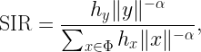
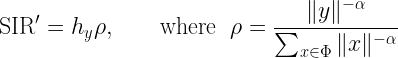
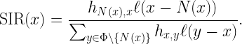
To this end, we focus on a downlink cellular setting where BSs form a stationary point process Φ and a user and a passive IRS with N elements are placed in each (Voronoi) cell. The exact distribution is irrelevant for our purposes. The desired signal at each user consists of the direct signal from its BS plus the intelligently reflected signal at its IRS. The SIR of a user at the origin served by the BS at x0 can be expressed as
where ℓ(x0) is the path loss from the serving BS and
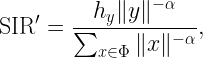
Here the random variables g0 and gi capture the (amplitude) fading over the direct link and reflected (indirect) link respectively, and the triangle parameter Δ captures the distances in the BS-IRS-user triangle. For details, please see this paper. The pertinent question is what constitutes the interference I. If all BSs are active, their interference is
But how about the IRSs? This is where it becomes contentious. Some argue that the IRSs emit signals and thus cause extra interference that is not captured in this sum over the BSs only. This would mean that we need to add a sum over the IRSs of the form
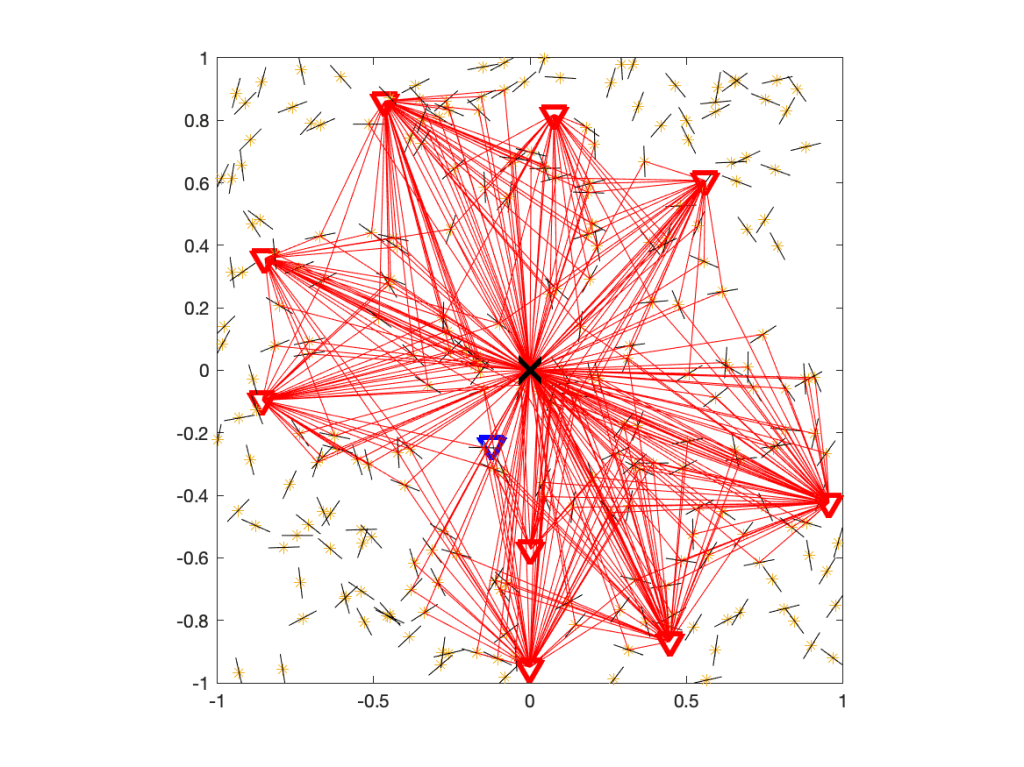
where Ψ is the point process of IRSs and pz is the power emitted by the IRS located at z. To decide whether Q is real or fake, let us have a look at the underlying network model. With fading modeled as Rayleigh, it is understood that the propagation of all signals is subject to rich scattering, i.e., there is multi-path propagation. For the case without IRSs, the propagation of interfering signals is illustrated here:
Figure 1. Propagation in a rich scattering environment without IRSs.
Figure 1 shows the user at the origin, its serving BS (blue triangle), and the interfering BSs (red triangles). The small black lines indicate scattering and reflecting objects. Some of the paths from interfering BSs via scattering objects to the user are shown with 319 red lines.
Now, let’s add one IRS per interfering BS. The resulting propagation environment is shown in Figure 2.
Figure 2. Propagation in a rich scattering environment with IRSs.
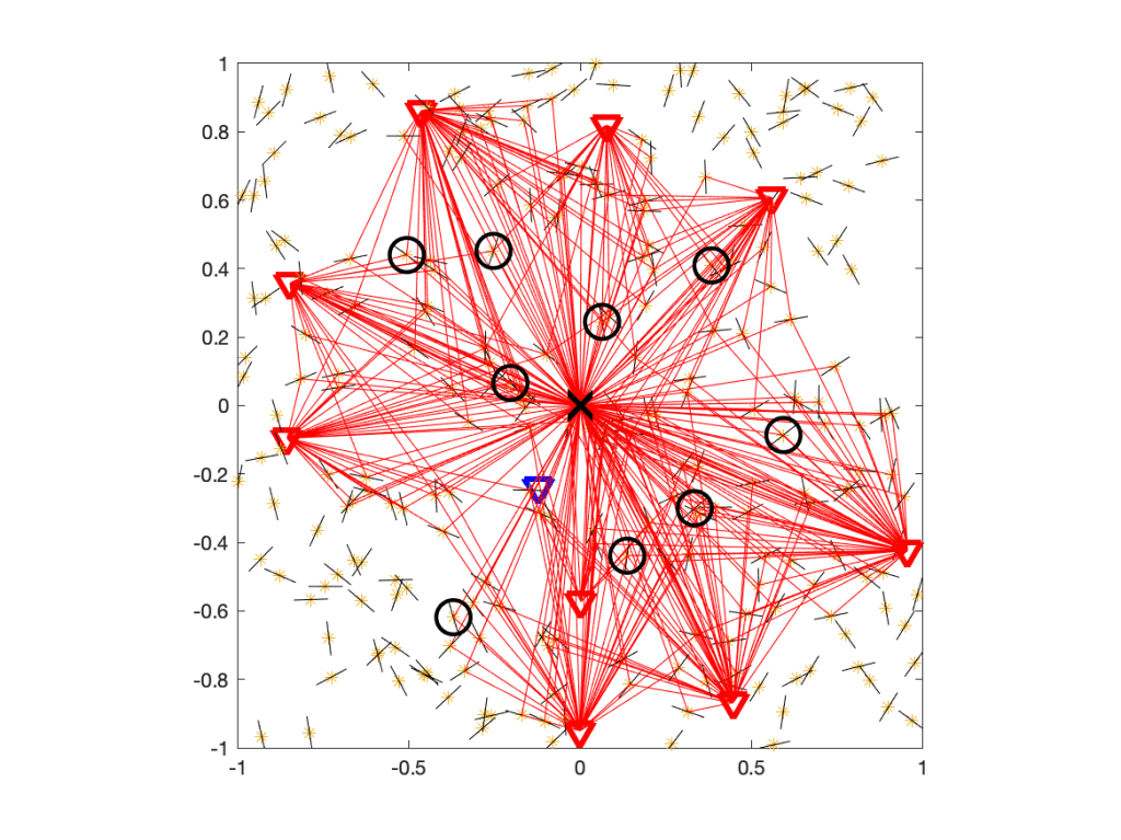
From the perspective of the user at the origin, the IRSs are unmatched, which means they act just like any of the other scattering and reflecting objects. So the difference to the IRS-free case is that there is a tiny fraction of additional scatterers, as highlighted in Figure 3.
Figure 3. Same as Figure 2, but with the IRSs encircled.
In this case, the IRSs add 4% to the scattering objects. If we did raytracing, they could make a small difference. In analytical work where the fading model is based on the assumption of a large number of scatterers, with the number of propagation paths tending to infinity, they make no difference at all. So we conclude that there is no extra interference Q due to the presence of passive IRSs and thus I=IBS. The signals reflected at unmatched IRSs are no different from signals reflected at any other object, and multi-path fading models already incorporate all such reflections.
Another argument that IRSs cannot cause extra interference is based on the fundamental principle of energy conservation. If Q did exist, its mean would be proportional to the density of IRSs deployed. This implies that there would be a density of IRSs beyond which the “interference” from the IRSs exceeds the total power transmitted by all BSs, which obviously is not physically possible.
In performance analyses of wireless networks, we frequently encounter expectations of the form
called average (ergodic) spectral efficiency (SE) or mean normalized rate or similar, in units of nats/s/Hz. For networks models with uncertainty, its evaluation requires the use stochastic geometry. Sometimes the metric is also normalized per area and called area spectral efficiency. The SIR is expressed in the form
with Φ being the point process of interferers. There are several underlying assumption made when claiming that (*) is a relevant metric:
It is assumed that codewords are long enough and arranged in a way (interspersed in time, frequency, or across antennas) such that fading is effectively averaged out. This is reasonable for several current networks.
It is assumed that desired signal and interference amplitudes are Gaussian. This is sensible since if a decoder is intended for Gaussian interference, then the SE is as if the interference amplitude were indeed Gaussian, regardless of its actual distribution.
Most importantly and questionably, taking the expectation over all fading random variables hx implies that the receiver has knowledge of all of them. Gifting the receiver with all the information of the channels from all interferers is unrealistic and thus, not surprisingly, leads to (*) being a loose upper bound on what is actually achievable.
So what is a more realistic and accurate approach? It turns out that if the fading in the interferers’ channels is ignored, i.e., by considering
we can obtain a tight lower bound on the SE instead of a loose upper bound. A second key advantage is that this formulation permits a separation of temporal and spatial scales, in the sense of the meta distribution. We can write
is a purely geometric quantity that is fixed over time and cleanly separated from the time-varying fading term hy. Averaging locally (over the fading), the SE follows as
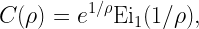
which is a function of (conditioned on) the point process. For instance, with Rayleigh fading,
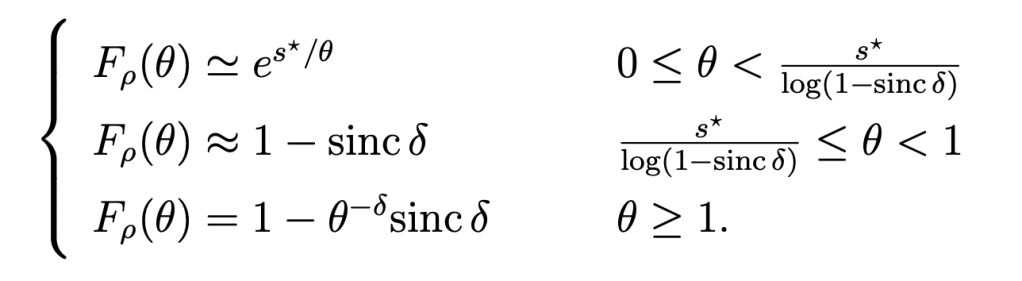
where Ei1 is an exponential integral. The next step is to find the distribution of ρ to calculate the spatial distribution of the SE – which would not be possible from (*) since it is an “overall average” that lumps all randomness together. In the case of Poisson cellular networks with nearest-base station association and path loss exponent 2/δ, a good approximation is
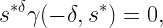
Here s* is given by
and γ is the lower incomplete gamma function. This approach lends itself to extensions to MIMO. It turns out that the resulting distribution of the SE is approximately lognormal, as illustrated in Fig. 1.
Figure 1: Spatial distribution of ergodic spectral efficiency for 2×2 MIMO in a Poisson cellular network and its lognormal approximation (red).
For SISO and δ=1/2 (a path loss exponent of 4), this (approximative) analysis shows that the SE achieved in 99% of the network is 0.22 bits/s/Hz, while a (tedious) simulation gives 0.24 bits/s/Hz. Generally, for small ξ, 1/ln(1/ξ) is achieved by a fraction 1-ξ of the network. As expected from the discussion above, this is a good lower bound.
In contrast, using the SIR distribution directly (and disregarding the separation of temporal and spatial scales), from
we would obtain an SE of only log2(1.01)=0.014 bits/s/Hz for 99% “coverage”, which is off by a factor of 16! So it is important that coverage be gleaned from the ergodic SE rather than a quantity subject to the small-scale variations of fading. See also this post.
The take-aways for the ergodic spectral efficiency are:
Avoid mixing time and spatial scales by expecting first over the fading and separately over the point process; this way, the spatial distribution of the SE can be obtained, instead of merely its average.
Avoid gifting the receiver with information it cannot possibly have; this way, tight lower bounds can be obtained instead of loose upper bounds.
Intuition may tell us that increasing the randomness in the system (e.g., by increasing the variance of some random variables relative to their mean) will decrease the correlation between some random quantities of interest. A prominent example is the interference or SIR in a wireless network measured at two locations or in two time slots.
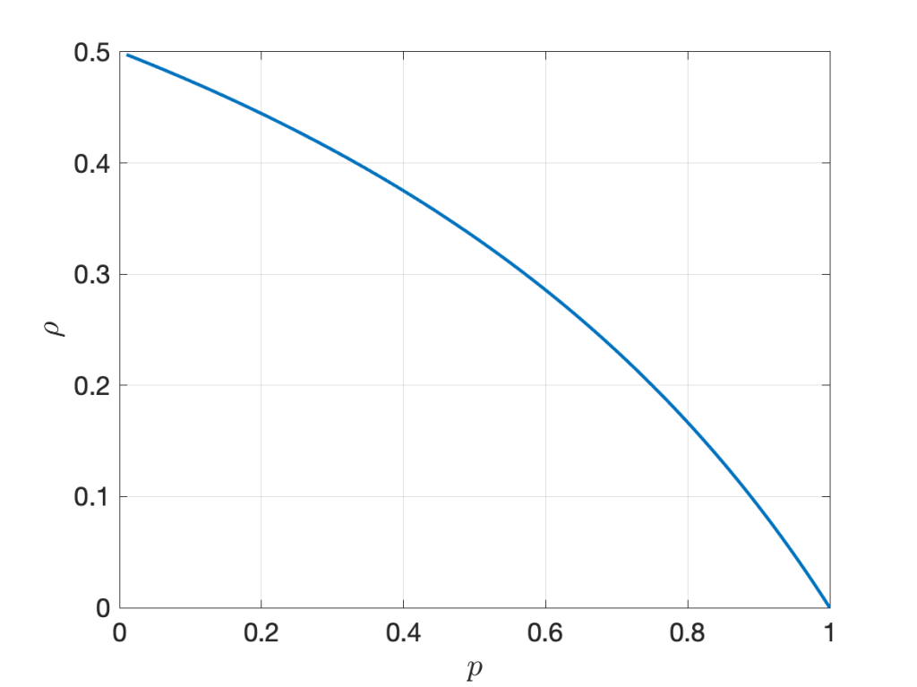
Let us consider a simple example to explore whether this intuition is correct. We consider the two random variables XY1 and XY2, where Y1 and Y2 are iid exponential with mean 1 and X is Bernoulli with mean p, independent of the Yk. In this case, Pearson’s correlation coefficient is
It is illustrated in Figure 1 below. The randomness in X, measured by the ratio of variance to mean, is 1-p . However, increasing the randomness monotonically increases the correlation. As p approaches 0, the correlation tends to its maximum of 1/2.
Figure 1: Correlation coefficient of XY1 and XY2 where X is Bernoulli(p) and Yk are iid exponential(1).
Next, let Y1 and Y2 be independent and Bernoulli with mean p and X gamma distributed with parameters m and 1/m, such that the mean of X is 1 and the variance 1/m. Again we focus on the correlation of the two products XY1 and XY2. In this case, the correlation coefficient is
shown in Figure 2 below for different values of m. Again, we observe that increasing the randomness in X (decreasing m) increases the correlation for all p <1. For p =1, the correlation is 1 since both random variables equal X.
Figure 2: Correlation coefficient of XY1 and XY2 where X is gamma(m,1/m) and Yk are iid Bernoulli(p).
So is the relationship between randomness and correlation completely counter-intuitive? Not quite, but our intuition is probably skewed towards the case of independent randomness, as opposed to common randomness. In the second example, the randomness in Y1 and Y2 decreases with p, and the correlation coefficient increases with p, as expected. Here Y1 and Y2 are independent. In contrast, X is the common randomness. If its variance increases, the opposite happens – the randomness decreases.
In the wireless setting, the common randomness is often the point process of transceiver locations, while the independent randomness usually comprises the fading coefficients and the channel access indicators. One of the earliest results on correlations in wireless networks is the following: For transmitters forming a PPP, with each one being active independently with probability p in each time slot (slotted ALOHA) and independent Nakagami-m fading, the correlation coefficient of the interference measured at the same location in two different time slots is (see Cor. 2 in this paper)
Here the fading coefficients have the same gamma distribution as in the second example above. As expected, increasing the randomness in the channel access (decreasing p) and in the fading (decreasing m) both reduce the correlation. Conversely, setting p =1 and letting m → ∞, the correlation coefficient is 1. However, the correlation is induced by the PPP as the common randomness – if the node placement was deterministic, the correlation would be 0. In other words, the interference in different times slots is conditionally independent given the PPP. This conditional independence is exploited in the analysis of important metrics such as the local delay and the SIR meta distribution.
One last remark. The expression (*) shows that the correlation coefficient is simply the product of the transmit probability p and the Nakagami fading parameter m mapped to the (0,1) interval using the Möbius homeomorphic transform described here, which is m /(m+1). This shows a nice symmetry in the impact of channel access and fading.
When simulating a point process to characterize the performance of the typical point (typical user or receiver), a conditioned version of the point process given a point at the origin o may not be available. It is then tempting to choose the “next best” point as a substitute, which may be the point closest to the origin. (Whether the coordinates are then shifted so that this point is at o is irrelevant.) The goal of this post is to show that this point is not typical, i.e., producing many realizations of the point process and evaluating the performance at this point does not yield the performance of the typical point. I call the point closest to o after averaging over the point process the 0-point. Put differently, the 0-point is the typical point among all points closest to o across the realizations of the point process. In a cellular network, the 0-point is the nucleus of the 0-cell (see this post), hence the term.
For simplicity, let us consider the homogeneous PPP of intensity 1 and focus on the probability that a disk of radius r centered at a point contains no other points, which we refer to as the NOPID (no other point in disk) probability. Equivalently, it is the probability that the nearest neighbor is at distance at least r. For the typical point, the NOPID probability is exp(-πr2). For the 0-point, let D be its distance from o. Given D, the disk of radius D centered at o, denoted as b(o,D), is empty, so the points excluding the 0-point form a PPP on ℝ2\b(o,D), and the NOPID probability is the probability that b((D,0),r)\b(o,D) is empty. This region is shown in blue in the movie below for different r given that the 0-point is at (1,0), i.e., D=1. For r<2D, it is moon- or crescent-shaped, while for r>2D, it is a disk with a hole.
Movie: Illustration of relevant region for the NOPID probability of the 0-point.
Letting A(r,d)=|b((d,0),r)\b(o,d)|, the (unconditioned) NOPID probability is 𝔼(exp(-A(r,D)), where D is Rayleigh distributed with mean 1/2. It can be expressed as
where
is the area A(r,d) for r<2d. For r>2d, A(r,d)=π(r2–d2), which results in the first term in (1).
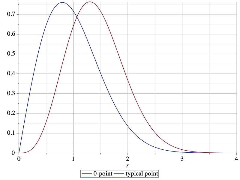
The NOPID probabilities of the 0-point and the typical point are compared below. It is apparent that the 0-point is more isolated than the typical point.
Figure: Comparison of NOPID probabilities.
By integrating the NOPID probability of the 0-point, we obtain the mean nearest-neighbor distance as 0.5953. This is almost 20% larger than that of the typical point, which is 1/2. The difference between the two NOPID probabilities is not just in the mean, though. They differ qualitatively in the tail. For large r, it follows from (1) that the ratio of the two NOPID probabilities approaches πr2/4. This implies that a Rayleigh distribution with adjusted mean will not provide a good fit to the NOPID probability at the 0-point.
The difference is even more pronounced if we consider directional nearest neighbors. If we consider a sector of angle π/2, then the nearest neighbor of the typical point is at distance 1 on average, irrespective of the orientation of the sector. For the 0-point, in the direction opposite from o, the mean distance is also 1, since on that side, the PPP is unaffected by the empty disk b(o,D). In the direction towards o, however, the distance is significantly larger, with a mean of 1.4205. The plot below shows the pdf of the directional nearest-neighbor distance of the 0-point oriented towards o (red) and the pdf of the directional nearest-neighbor distance of the typical point (blue), given by (π/2)r exp(-(π/4)r^2). The pdfs are the negative derivatives of the NOPIS (no other point in sector π/2) probabilities.
Figure: pdf of the distance to the directional nearest neighbor of the 0-point in π/2 sector oriented towards o, in comparison with that of the typical point.
When applied to cellular networks (with nearest-base station association), the 0-point is the base station serving the typical user (at o). The discussion here reveals that the 0-base station behaves differently from the typical base station. In particular, the point process of the other base stations viewed from the 0-base station is highly non-isotropic. In the direction of the typical user, the nearest other base station is much further away than in the opposite direction. This fact is consistent with the conclusions from this post on the shape of the 0-cell in the Poisson-Voronoi tessellation.
The analysis of cellular networks usually focuses on the typical user in the downlink and the typical base station (or, equivalently, the typical cell) in the uplink. It is important that if base station and user point processes are independent, the two notions of “typical” are not compatible – the typical user’s cell is statistically different from the typical cell. The difference is caused by the effect of size-biased sampling. The typical user’s performance corresponds to that of the average of all users, and there are more users in larger cells. Since a user model is not needed in the downlink as explained in this post, we can equivalently say that an arbitrary location is more likely to fall in a larger cell than a smaller cell. The typical user’s cell, the so-called 0-cell, is the cell containing the origin, i.e., it is obtained by cell area-biased sampling, which gives larger cells more weight. As a result, the 0-cell is larger on average than the typical cell, which is the cell of the base station conditioned to be at the origin. The statistical properties of the typical cell correspond to the averages of all cells.
Such size-biased sampling is not restricted to cellular networks or stochastic geometry. If we throw a dart blindly on a world map until we hit land, the country we hit is quite likely to be a big one. In fact, there is a 50% chance that the dart lands on one of the 10 largest countries. Similarly, the typical country has 40 M inhabitants on average, but the typical person is likely to live in a country with more than 100 M people. The typical dollar is quite likely owned by a wealthy person, while the typical person is probably not rich. The typical human hair is likely to grow on a person with full hair, while the typical person has a 5-10% chance of being bald. The typical animal leg has a decent chance of belonging to a millipede or centipede, while the typical animal is very unlikely to have more than six feet.
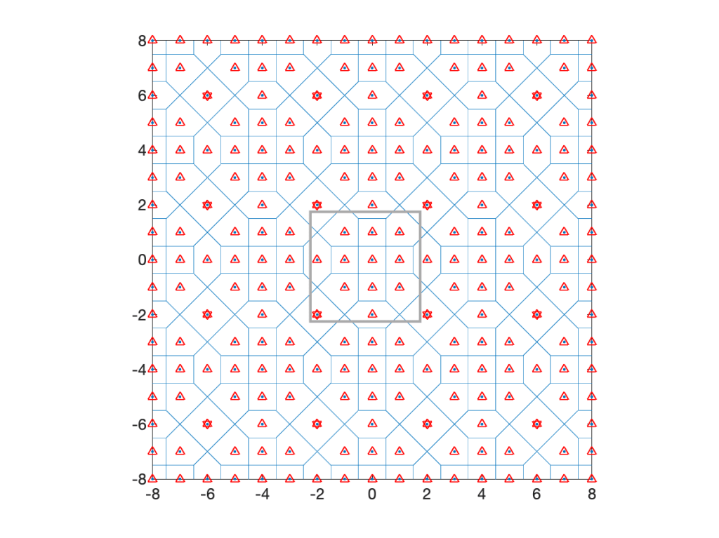
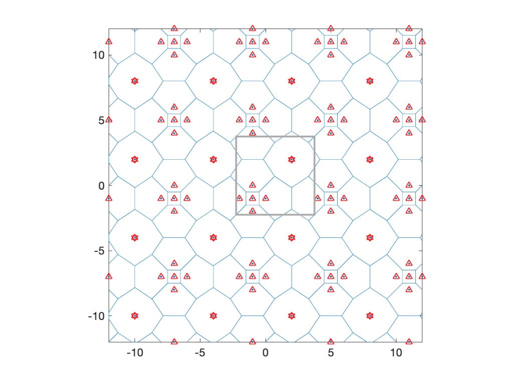
Coming back to cellular networks, let us focus on a concrete example that is fully tractable in terms of the cell area distributions. Consider the lattice with holes shows in Fig. 1 below, obtained from a square lattice of density 1 by removing the four nearest neighbors of each 16th point. It is periodic with period 4 in both directions, its density is λ=3/4, and it has four different types of cells, with three different areas, 1, 3/2, and 2.
Fig. 1: Lattice hole process with density 3/4. Base stations (cell nuclei) are marked by red triangles, and those whose nearest neighbors were removed by stars, which makes these cell large. The grey box indicates one period of the lattice.
The typical cell has area 1 with probability 5/12, area 3/2 with probability 1/2, and area 2 with probability 1/12. The mean area follows as E(A)=5/12+1/2 3/2+1/12 2=4/3, which corresponds to 1/λ.
Now assume a stationary square lattice of density 1 as the user point process. Then the cells of area 1 always contain 1 user and those of area 2 always contain 2 users. Those of area 3/2 have 1 user or 2 users, each with probability 1/2. Deconditioning on the cell areas, we obtain the distribution of the number of users U in the typical cell as P(U=1)=2/3 and P(U=2)=1/3, for a mean number of users E(U)=4/3, which equals the mean area times the user density (chosen to be 1 here).
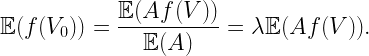
How about the typical user’s cell? This is where the size bias plays a role. The distribution of the area A0 of the 0-cell is P(A0=1)=5/16, P(A0=3/2)=9/16, and P(A0=2)=1/8. These are the fractions of the plane covered by cells of areas 1, 3/2, and 2. The mean area is E(A0)=45/32, which is about 5.5% bigger than the mean area of the typical cell. The number of users U0 in the 0-cell is distributed as P(U0=1)=5/16+1/2 9/16=19/32, P(U0=2)=1/2 9/16+1/8=13/32, resulting in a mean of E(U0)=45/32, which is the user density times the mean area. The mean also follows from the general formula
where V is the typical cell, V0 the 0-cell, and f is a non-negative function on compact sets. Applied to our setting, where f(V) is the number of users in V, we obtain
Since the user density is 1, this is also the mean area of A0. For the number of sides S, we have E(S)=19/4, but E(S0)=155/32, which is bigger by 3/32. At the end of this post are three more examples of similarly constructed lattices. In each case, the points within a certain distance of a sub-lattice are removed.
So the typical user is not served by the typical base station, and the typical base station does not serve the typical user. One way to reconcile the two is to define a user point process where a fixed number of users, say one, is placed uniformly at random in each cell. Such a user process is of course no longer independent of the base station process.
For Poisson distributed base stations, the 0-cell is 28% larger than the typical cell. Its mean number of sides is 6.41, whereas the typical cell has 6 sides on average. Hence the 0-cell is not just an enlarged version of the typical cell but also has a different shape. Accordingly, the distance from the nucleus of the typical cell to a random point in the cell is not Rayleigh distributed as it is in the 0-cell. Also, if users form a PPP of density 1, the typical user’s cell has 1+1.28/λ users on average (there is one extra user due to the conditioning of a user to be at the origin), while the typical cell only has a mean of 1/λ users.
Size-biased sampling is important in other wireless networks as well. If a vehicular network is modeled by placing one-dimensional Poisson point processes (cars) on line segments (streets) of independent random length (which is a Cox process supported on line segments), then the typical vehicle’s street length distribution fL0 is different from the length distribution f_L of the streets. By length-biased sampling, the two are related as
For example, if L is exponential with mean 1, then L0 is gamma distributed with mean 2. The same situation arises in the interarrival intervals of a one-dimensional PPP (of density 1). The typical such interval is exponential with mean 1, but the interval containing the origin (or any other deterministic time instant) has a mean length of 2. This is sometimes referred to as the waiting time paradox, although there is nothing paradoxical about it – it is just size-biased sampling.
Lastly, as promised, here are three more examples of lattices with increasingly large holes.
Fig. 2: Lattice with period 6. λ=1/6; P(A=1)=1/6; P(A=89/15)=2/3; P(A=169/15)=1/6; E(A)=6. P(A0=1)=1/36; P(A0=89/15)=89/135; P(A0=169/15)=169/540; E(A0)=6047/810 ≈ 7.46.Fig. 3: Lattice with period 8. λ=7/32; P(A=1)=5/14; P(A=7/2)=2/7; P(A=29/4)=2/7; P(A=16)=1/14; E(A)=32/7. P(A0=1)=5/64; P(A0=7/2)=7/32; P(A0=29/4)=29/64; P(A0=16)=1/4; E(A0)=2081/256. Here the 0-cell is almost twice as big on average than the typical cell. It corresponds to the largest cell with probability 1/4, but only 1/14 of the cells are largest ones.Fig. 4: Lattice with period 16. λ=7/128; P(A=1)=5/14; P(A=15/2)=2/7; P(A=33)=2/7; P(A=89)=1/14; E(A)=128/7. P(A0=1)=5/256; P(A0=15/2)=15/128; P(A_0=33)=33/64; P(A0=89)=89/256; E(A0)=12507/256 ≈ 48.9. The 0-cell is more than 2.5 times larger than the typical one on average.
Let us consider the downlink of a cellular network where base stations form a stationary and ergodic point process Φ and define the SIR at each location x ∈ R2 as
Here N(x) is the nucleus of the Voronoi cell that x belongs to, hx,y is the fading coefficient between x and y, and ℓ is the path loss function. Due to the stationarity of Φ, the SIR statistics do not depend on the location x. In other words, any arbitrary location can be taken to be the typical location that the analysis focuses on. Example result: If Φ is Poisson, the fading is Rayleigh, and ℓ is a power-law function with exponent 2/δ, it is known that for all x ∈ R2,
where 2F1 is the Gauss hypergeometric function. Since Φ is ergodic, the probability that the SIR exceeds θ is the fraction of the plane that achieves an SIR of at least θ for all realizations of Φ. This means that the probability (ensemble average) can be replaced by a spatial average over an increasingly large region. Sometimes this probability (or spatial average) is questionably called “coverage probability” (see this post), and the area fraction is termed “covered area fraction”. It is important to note that results such as (1) do not require any specification of a point process of users. This answers the question in the title: No, users are not necessary in the downlink SIR analysis.
That said, in the literature we observe that in many cases, a point process of users is defined before such downlink SIR results are derived. The reason could be that it may seem overly abstract to consider a cellular network model devoid of any users and view the SIR as a random field on the plane. Specializing the location x to the points of a user point process (assumed independent of Φ), we observe that (1) is the SIR distribution at the typical user for any stationary point process of users. So there is nothing wrong in introducing a point process of users, focus on the typical user, and state a result such as (1). It would, however, be potentially misleading to specify the user point process to be a Poisson process, since the reader may then believe that the result only holds for Poisson distributed users.
There is one caveat when introducing a point process of users to formulate downlink results: The interpretation of the SIR distribution as the fraction of users who achieve SIR>θ in each realization of the user and base station point processes may no longer be correct, even if the two point processes are independent and stationary and ergodic. For instance, consider the case where both are stationary (i.e., randomly translated) lattices of the same intensity. Then, given the point processes, the SIR distribution at each user is the same and depends on the relative shift of the lattices. For example, if a user is very close to its serving base station, then all users are close to their serving base station, and the SIR at all users is likely to exceed θ even when θ is, say, 20 dB. In contrast, if one user is equidistant to two base stations, then all users are, and it is unlikely that the SIR (at any or all of them) exceeds 1. So averaging over the users in one realization cannot yield the same result as averaging over the point processes (ensemble averaging). But doesn’t ergodicity imply that the two results are the same? The answer is yes, it does, but individual ergodicity of the two point processes is not sufficient. Since the SIR depends on both of them jointly, they need to be jointly ergodic. This is the condition that is not met in this example scenario of two lattices.
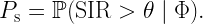
The fraction of reliable links is an important metric, in particular for applications with (ultra-)high reliability requirements. In the literature, we see that it is sometimes equated with the transmission success probability of the typical link, given by
This is the SIR distribution (in terms of the complementary cdf) at the typical link. In this post I would like to discuss whether it is accurate to call ps the fraction of reliable links.
Say someone claims “The fraction of reliable links in this network is ps=0.8″, and I ask “But how reliable are these links?”. The answer might be “They are (at least) 80% reliable of course, because ps=0.8.” Ok, so let us assume that the fraction links with reliability at least 0.8 is 0.8. Following the same logic, the fraction of links with reliability at least 0.7 would be 0.7. But clearly that fraction cannot be smaller than the fraction of links with reliability at least 0.8. There is an obvious contradiction. So how can we quantify the fraction of reliable links in a rigorous way?
First we note that in the expression for ps, there is no notion of reliability but ps itself. This leads to the wrong interpretation above that a fraction ps of links has reliability at least ps. Instead, we want so specify a reliability threshold so that we can say, e.g., “the fraction of links that are at least 90% reliable is 0.8”. Naturally it then follows that the fraction of links that are at least 80% reliable must be larger than (or equal to) 0.8. So a meaningful expression for the fraction of reliable links must involve a reliability threshold parameter that can be tuned from 0 to 1, irrespective of how reliable the typical link happens to be.
Second, ps gives no indication about the reliability of individual links. In particular, it does not specify what fraction of links achieve a certain reliability, say 0.8. It could be all of them, or 2/3, or 1/2, or 1/5. ps=0.8 means that the probability of transmission success over the typical link is 0.8. Equivalently, in an ergodic setting, in every time slot, a fraction 0.8 of all links happens to succeed, in every realization of the point process. But some links will be highly reliable, while others will be less reliable.
Before getting to the definition of the fraction of reliable links, let us focus on Poisson bipolar networks for illustration, with the following concrete parameters: link distance 1/4, path loss exponent 4, target SIR threshold θ=1, and the fading is iid Rayleigh. The link density is λ, and we use slotted ALOHA with transmit probability is p. In this case, the well-known expression for ps is
where c=0.3084 is a function of link distance, path loss exponent, and SIR threshold. We note that if we keep λp constant, ps remains unchanged. Now, instead of just considering the typical link, let us consider all the links in a realization of the network, i.e., for a given set of locations of all transceivers. The video below shows the histogram of the individual link reliabilities for constant λp=1 while varying the transmit probability p from 1.00 to 0.01 in steps of 0.01. The red line indicates ps, which is the average of all link reliabilities and remains constant at 0.735. Clearly, the distribution of link reliabilities changes significantly even with constant ps – as surmised above, ps does not reveal how disparate the reliabilities are. The symbol σ refers to the standard deviation of the reliability distribution, starting at 0.3 at p=1 and decreasing to less than 1/10 of that for p=1/100.
Histogram of link reliabilities in bipolar network.
Equipped with the blue histogram (or pdf), we can easily determine what fraction of links achieves a certain reliability, say 0.6, 0.7, or 0.8. These are shown in the plot below. It is apparent that for small p, due to the concentration of the link reliabilities as p→0, the fraction of reliable links tends to 0 or 1, depending on whether the reliability threshold is above or below the average ps .
Fraction of links achieving reliability at least 0.6, 0.7, 0.8.
So how do we characterize the link reliability distribution theoretically? We start with the conditional SIR ccdf at the typical link, given the point process:
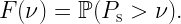
Then ps=E(Ps), with the expectation taken over the point process. Hence ps is the mean of the conditional success probability, and if we consider its distribution, we arrive at the link reliability distribution, shown in blue in the video above. Mathematically,
where ν is the target reliability. This distribution is a meta distribution, since it is the distribution of a conditional distribution. In ergodic settings, it specifies the fraction of links that achieve an SIR of θ with reliability at least ν, which is exactly what we set out to quantify. In conclusion: The fraction of reliable links is not given by the standard (mean) success probability; it is given by the meta distribution of the SIR.
The concept of the typical point is important in point process theory. In the wireless context, it is often concretized to the typical user, typical receiver, typical vehicle, etc. The typical point is an abstraction in the sense that it is not a point that is selected in any deterministic fashion from the point process, neither is it an arbitrary point. Also, speaking of “a typical point” is misleading, since it suggests that there exist a number of such typical points in the process (or perhaps even in a realization thereof), and we can choose one of them to “obtain a typical point”. This does not work – there is nothing “typical” about a point selected in a deterministic fashion, let alone an arbitrary point. That said, if the total number of points is finite, we can, loosely speaking, argue that the typical point is obtained by choosing one of the points uniformly at random. Even this is not trivial since picking a point in a single realization of the point process does generally not produce the desired result, for example of the point process is not ergodic. Many realizations need to be considered, but then the question arises how exactly to pick a point uniformly from many realizations. If the number of points is infinite, any attempt of picking a point uniformly at random is bound to fail because there is no way to select a point uniformly from infinitely many, in much the same way that we cannot select an integer uniformly at random.
So how do we arrive at the typical point? If the point process is stationary and ergodic, we can generate the statistics of the typical point by averaging those of each individual point in a single realization, observed in an increasingly large observation window. This leads to the interpretation of the typical point as a kind of “average point”. Similarly, we may find that the “typical American male” weighs 89.76593 kg, which does not imply that there exists an individual with that exact weight but means that if we weighed every(male)body or a large representative sample, we would obtain that average weight. For general (stationary) point processes, we obtain the typical point by conditioning on a point to exist at a certain location, usually the origin o. Upon averaging over the point process (while holding on to this point at the origin), that point becomes the typical point. The distribution of this conditioned point process is the Palm distribution. In the case of the Poisson process, conditioning on a point at o is the same as adding a point at o. This equivalence is called Slivnyak’s theorem.
In the non-stationary case, the typical point at location x may have different statistical properties than the typical point at another location y. As a result, there exist Palm measures (or distributions) for each location in the support of the point process. In this case, the formal definition of the Palm measure is given by the Radon-Nikodym derivative (with respect to the intensity measure) of the Campbell measure. In the Poisson case, Slivnyak’s theorem still applies.