Month: January 2021

The point closest to the origin is not typical

When simulating a point process to characterize the performance of the typical point (typical user or receiver), a conditioned version of the point process given a point at the origin o may not be available. It is then tempting to choose the “next best” point as a substitute, which may be the point closest to the origin. (Whether the coordinates are then shifted so that this point is at o is irrelevant.) The goal of this post is to show that this point is not typical, i.e., producing many realizations of the point process and evaluating the performance at this point does not yield the performance of the typical point. I call the point closest to o after averaging over the point process the 0-point. Put differently, the 0-point is the typical point among all points closest to o across the realizations of the point process. In a cellular network, the 0-point is the nucleus of the 0-cell (see this post), hence the term.

For simplicity, let us consider the homogeneous PPP of intensity 1 and focus on the probability that a disk of radius r centered at a point contains no other points, which we refer to as the NOPID (no other point in disk) probability. Equivalently, it is the probability that the nearest neighbor is at distance at least r. For the typical point, the NOPID probability is exp(-πr2). For the 0-point, let D be its distance from o. Given D, the disk of radius D centered at o, denoted as b(o,D), is empty, so the points excluding the 0-point form a PPP on ℝ2\b(o,D), and the NOPID probability is the probability that b((D,0),r)\b(o,D) is empty. This region is shown in blue in the movie below for different r given that the 0-point is at (1,0), i.e., D=1. For r<2D, it is moon- or crescent-shaped, while for r>2D, it is a disk with a hole.

Movie: Illustration of relevant region for the NOPID probability of the 0-point.

Letting A(r,d)=|b((d,0),r)\b(o,d)|, the (unconditioned) NOPID probability is 𝔼(exp(-A(r,D)), where D is Rayleigh distributed with mean 1/2. It can be expressed as

\displaystyle \qquad\qquad F_0(r)=\frac{\pi}{4}r^2 e^{-\pi r^2}+\int_{r/2}^\infty e^{-A'(r,u)}2\pi u e^{-\pi u^2}{\rm d}u,\qquad\qquad (1)

where

\displaystyle A'(r,d)=\pi r^2-r^2\cos^{-1}\left(\frac{r}{2d}\right)-d^2\cos^{-1}\left(1-\frac{r^2}{2d^2}\right)+\frac{r}{2}\sqrt{4d^2-r^2}.

is the area A(r,d) for r<2d. For r>2d, A(r,d)=π(r2d2), which results in the first term in (1).

The NOPID probabilities of the 0-point and the typical point are compared below. It is apparent that the 0-point is more isolated than the typical point.

Figure: Comparison of NOPID probabilities.

By integrating the NOPID probability of the 0-point, we obtain the mean nearest-neighbor distance as 0.5953. This is almost 20% larger than that of the typical point, which is 1/2. The difference between the two NOPID probabilities is not just in the mean, though. They differ qualitatively in the tail. For large r, it follows from (1) that the ratio of the two NOPID probabilities approaches πr2/4. This implies that a Rayleigh distribution with adjusted mean will not provide a good fit to the NOPID probability at the 0-point.

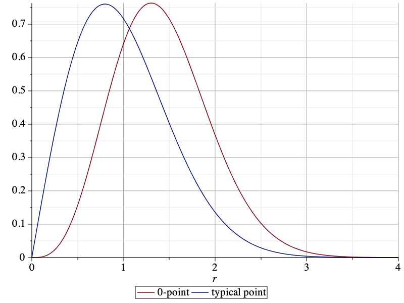
The difference is even more pronounced if we consider directional nearest neighbors. If we consider a sector of angle π/2, then the nearest neighbor of the typical point is at distance 1 on average, irrespective of the orientation of the sector. For the 0-point, in the direction opposite from o, the mean distance is also 1, since on that side, the PPP is unaffected by the empty disk b(o,D). In the direction towards o, however, the distance is significantly larger, with a mean of 1.4205. The plot below shows the pdf of the directional nearest-neighbor distance of the 0-point oriented towards o (red) and the pdf of the directional nearest-neighbor distance of the typical point (blue), given by (π/2)r exp(-(π/4)r^2). The pdfs are the negative derivatives of the NOPIS (no other point in sector π/2) probabilities.

Figure: pdf of the distance to the directional nearest neighbor of the 0-point in π/2 sector oriented towards o, in comparison with that of the typical point.

When applied to cellular networks (with nearest-base station association), the 0-point is the base station serving the typical user (at o). The discussion here reveals that the 0-base station behaves differently from the typical base station. In particular, the point process of the other base stations viewed from the 0-base station is highly non-isotropic. In the direction of the typical user, the nearest other base station is much further away than in the opposite direction. This fact is consistent with the conclusions from this post on the shape of the 0-cell in the Poisson-Voronoi tessellation.

The curious shape of Poisson-Voronoi cells

In this blog we are exploring the shape of two kinds of cells in the Poisson-Voronoi tessellation on the plane, namely the 0-cell and the typical cell. The 0-cell is the cell containing the origin, while the typical cell is the cell obtained by conditioning on a Poisson point to be at the origin (which is the same as adding the origin to the PPP).

The cell shape has an important effect on the signal and interference powers at the typical user (in the 0-cell) and at the user in the typical cell. For instance, in the 0-cell, which contains the typical user at a uniformly random location, about 1/4 of the cell edge is at essentially the same distance to the base station as the typical user on average). Hence it is not the case that edge users necessarily suffer from larger signal attenuation than the typical user (who resides inside the cell).

The cell shape is determined by the directional radii of the cells when their nucleus is at the origin. To have a well-defined orientation, we select a location uniformly in the cell and rotate the cell so that this location falls on the positive x-axis. In the 0-cell, this involves first a translation of the cell’s nucleus to the origin, followed by a rotation until the original origin (which is uniformly distributed in the cell) lies on the positive x-axis. This is illustrated in Movie 1 below. In the typical cell, it involves adding a Poisson point, selecting a uniform location, and a rotation so that this uniform location lies on the positive x-axis. This is illustrated in Movie 2.

Movie 1. Rotated and translated 0-cell.

Movie 2. Rotated typical cell.

As indicated in the movies, the distances from the nucleus to the uniformly random location are denoted by D0 and D, respectively, and the directional radii by R0(ϕ) and R(ϕ), respectively. This way, the boundary of the cells is described in polar coordinates as (R0(ϕ),ϕ) and (R(ϕ),ϕ), ϕ ∈ [0,2π). In a cellular network model, the uniform random location could be that of a user, while the PPP models the base stations. In this case D0 is the link distance from the typical user to its serving base station, while D is the link distance from the typical base station to a randomly located user it serves. The distinction between the typical user’s and the typical base station’s point of view is explained in this blog.

Let λ denote the density of the PPP. Three results are well known:

  • The distribution of D0 follows from the void probability of the PPP. It is Rayleigh with mean 1/(2√λ).
  • Since the mean area of the typical cell is 1/λ, we have ∫ 0π 𝔼(R(ϕ)2) dϕ = 1/λ.
  • The minimum of R(ϕ) is distributed with pdf f(r)=8λπr exp(-4λπr2). This is half the distance to the nearest neighboring Poisson point (base station).

In contrast, there is no closed-form expression for the distribution of D. Due to size-biased sampling, the area of the 0-cell stochastically dominates that of the typical cell and, in turn, D0 dominates D.

Analyzing the directional radii, we obtain these new insights on the cell shapes:

  • If Ψ is uniform in [0,π], R(Ψ) is again Rayleigh with mean 1/(2√λ).
  • R0(π) is also Rayleigh with the same mean. In fact, R0(π) and D0 are iid.
  • R0(0) has mean 3/(4√λ) and is distributed as

\displaystyle f_{R_0(0)}(y)=2(\lambda\pi)^2 y^3 \exp(-\lambda\pi y^2).

  • Hence R0(0) is on average exactly 50% larger than R0(π). For the typical cell, simulation results indicate that R(0) is about 55% larger on average than R(π).
  • The difference R0(0)-D0 is distributed as f(r)=π√λ erfc(r √(πλ)). Its mean is 1/(4√λ). Hence the typical user is no further from the cell edge than the base station on average.
  • The joint distribution of D0 and R0(ϕ) can be given in exact analytical form.
  • 3/4 of the typical cell is further away from the nucleus than the nearest point on the cell edge (i.e., the minimum directional radius). Expressed differently, a uniformly random user in the typical cell has a 75% chance of being further away from the base station than the nearest edge user. By simulation, D on average is 2.7 times larger than the minimum of the directional radii.

In conclusion, the 0-cell and the typical cell are quite asymmetric around the nucleus (base station) and the uniformly random point (user). In the direction away from the base station, the user is about 4 times closer to the cell edge than in the direction towards the base station, and many locations on the cell edge are closer to the base station than the user inside the cell. These results have implications on the design of efficient cellular network transmission schemes, such as beamforming, NOMA, and base station cooperation, in both down- and uplink.

More details are available in Section II of this paper.