In this post we contrast the meta distribution of the SIR with the standard SIR distribution. The model is the standard downlink Poisson cellular network with Rayleigh fading and path loss exponent 4. The base station density is 1, and the users form a square lattice of density 5. Hence there are 5 users per cell on average.
Fig. 1: The setup. Base stations are red crosses, and users are blue circles. They are served by the nearest base station. Cell boundaries are dashed.
We assume the base stations transmit to the users in their cell at a rate such that the messages can be decoded if an SIR of θ =-3 dB is achieved. If the user succeeds in decoding, it is marked with a green square, otherwise red. We let this process run over many time slots, as shown next.
Fig. 2: Transmission success (green) and failure (red) at each user over 100 time slots.
The SIR meta distribution captures the per-user statistics, obtained by averaging over the fading, i.e., over time. In the next figure, the per-user reliabilities are illustrated using a color map from pure red (0% success) to pure green (100% success).
Fig. 3: Per-user reliabilities, obtained by averaging over fading. These are captured by the SIR meta distribution. Near the top left is a user that almost never succeeds since it is equidistant to three base stations.
The SIR meta distribution provides the fractions of users that are above (or below) a certain reliability threshold. For instance, the fraction of users that are at least dark green in the above figure.
In contrast, the standard SIR distribution, sometimes misleadingly called “coverage probability”, is just a single number, namely the average reliability, which is close to 70% in this scenario (see, e.g., Eqn. (1) in this post). Since it is obtained by averaging concurrently over fading and point process, the underlying network structure is lost, and the only information obtained is the average of the colors in Fig. 3:
Fig. 4: The standard SIR distribution only reveals the overall reliability of 70%.
The 70% reliability is that of the typical user (or typical location), which does not correspond to any user in our network realization. Instead, it is an abstract user whose statistics correspond to the average of all users.
Acknowledgment: The help of my Ph.D. student Xinyun Wang in writing the Matlab program for this post is greatly appreciated.
In this blog we are exploring the shape of two kinds of cells in the Poisson-Voronoi tessellation on the plane, namely the 0-cell and the typical cell. The 0-cell is the cell containing the origin, while the typical cell is the cell obtained by conditioning on a Poisson point to be at the origin (which is the same as adding the origin to the PPP).
The cell shape has an important effect on the signal and interference powers at the typical user (in the 0-cell) and at the user in the typical cell. For instance, in the 0-cell, which contains the typical user at a uniformly random location, about 1/4 of the cell edge is at essentially the same distance to the base station as the typical user on average). Hence it is not the case that edge users necessarily suffer from larger signal attenuation than the typical user (who resides inside the cell).
The cell shape is determined by the directional radii of the cells when their nucleus is at the origin. To have a well-defined orientation, we select a location uniformly in the cell and rotate the cell so that this location falls on the positive x-axis. In the 0-cell, this involves first a translation of the cell’s nucleus to the origin, followed by a rotation until the original origin (which is uniformly distributed in the cell) lies on the positive x-axis. This is illustrated in Movie 1 below. In the typical cell, it involves adding a Poisson point, selecting a uniform location, and a rotation so that this uniform location lies on the positive x-axis. This is illustrated in Movie 2.
Movie 1. Rotated and translated 0-cell.Movie 2. Rotated typical cell.
As indicated in the movies, the distances from the nucleus to the uniformly random location are denoted by D0 and D, respectively, and the directional radii by R0(ϕ) and R(ϕ), respectively. This way, the boundary of the cells is described in polar coordinates as (R0(ϕ),ϕ) and (R(ϕ),ϕ), ϕ ∈ [0,2π). In a cellular network model, the uniform random location could be that of a user, while the PPP models the base stations. In this case D0 is the link distance from the typical user to its serving base station, while D is the link distance from the typical base station to a randomly located user it serves. The distinction between the typical user’s and the typical base station’s point of view is explained in this blog.
Let λ denote the density of the PPP. Three results are well known:
The distribution of D0 follows from the void probability of the PPP. It is Rayleigh with mean 1/(2√λ).
Since the mean area of the typical cell is 1/λ, we have ∫ 0π 𝔼(R(ϕ)2) dϕ = 1/λ.
The minimum of R(ϕ) is distributed with pdf f(r)=8λπr exp(-4λπr2). This is half the distance to the nearest neighboring Poisson point (base station).
In contrast, there is no closed-form expression for the distribution of D. Due to size-biased sampling, the area of the 0-cell stochastically dominates that of the typical cell and, in turn, D0 dominates D.
Analyzing the directional radii, we obtain these new insights on the cell shapes:
If Ψ is uniform in [0,π], R(Ψ) is again Rayleigh with mean 1/(2√λ).
R0(π) is also Rayleigh with the same mean. In fact, R0(π) and D0 are iid.
R0(0) has mean 3/(4√λ) and is distributed as
Hence R0(0) is on average exactly 50% larger than R0(π). For the typical cell, simulation results indicate that R(0) is about 55% larger on average than R(π).
The difference R0(0)-D0 is distributed as f(r)=π√λ erfc(r √(πλ)). Its mean is 1/(4√λ). Hence the typical user is no further from the cell edge than the base station on average.
The joint distribution of D0 and R0(ϕ) can be given in exact analytical form.
3/4 of the typical cell is further away from the nucleus than the nearest point on the cell edge (i.e., the minimum directional radius). Expressed differently, a uniformly random user in the typical cell has a 75% chance of being further away from the base station than the nearest edge user. By simulation, D on average is 2.7 times larger than the minimum of the directional radii.
In conclusion, the 0-cell and the typical cell are quite asymmetric around the nucleus (base station) and the uniformly random point (user). In the direction away from the base station, the user is about 4 times closer to the cell edge than in the direction towards the base station, and many locations on the cell edge are closer to the base station than the user inside the cell. These results have implications on the design of efficient cellular network transmission schemes, such as beamforming, NOMA, and base station cooperation, in both down- and uplink.
More details are available in Section II of this paper.
The analysis of cellular networks usually focuses on the typical user in the downlink and the typical base station (or, equivalently, the typical cell) in the uplink. It is important that if base station and user point processes are independent, the two notions of “typical” are not compatible – the typical user’s cell is statistically different from the typical cell. The difference is caused by the effect of size-biased sampling. The typical user’s performance corresponds to that of the average of all users, and there are more users in larger cells. Since a user model is not needed in the downlink as explained in this post, we can equivalently say that an arbitrary location is more likely to fall in a larger cell than a smaller cell. The typical user’s cell, the so-called 0-cell, is the cell containing the origin, i.e., it is obtained by cell area-biased sampling, which gives larger cells more weight. As a result, the 0-cell is larger on average than the typical cell, which is the cell of the base station conditioned to be at the origin. The statistical properties of the typical cell correspond to the averages of all cells.
Such size-biased sampling is not restricted to cellular networks or stochastic geometry. If we throw a dart blindly on a world map until we hit land, the country we hit is quite likely to be a big one. In fact, there is a 50% chance that the dart lands on one of the 10 largest countries. Similarly, the typical country has 40 M inhabitants on average, but the typical person is likely to live in a country with more than 100 M people. The typical dollar is quite likely owned by a wealthy person, while the typical person is probably not rich. The typical human hair is likely to grow on a person with full hair, while the typical person has a 5-10% chance of being bald. The typical animal leg has a decent chance of belonging to a millipede or centipede, while the typical animal is very unlikely to have more than six feet.
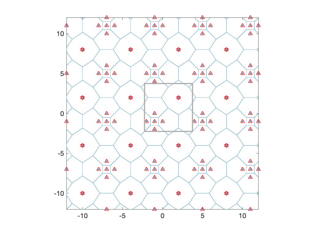
Coming back to cellular networks, let us focus on a concrete example that is fully tractable in terms of the cell area distributions. Consider the lattice with holes shows in Fig. 1 below, obtained from a square lattice of density 1 by removing the four nearest neighbors of each 16th point. It is periodic with period 4 in both directions, its density is λ=3/4, and it has four different types of cells, with three different areas, 1, 3/2, and 2.
Fig. 1: Lattice hole process with density 3/4. Base stations (cell nuclei) are marked by red triangles, and those whose nearest neighbors were removed by stars, which makes these cell large. The grey box indicates one period of the lattice.
The typical cell has area 1 with probability 5/12, area 3/2 with probability 1/2, and area 2 with probability 1/12. The mean area follows as E(A)=5/12+1/2 3/2+1/12 2=4/3, which corresponds to 1/λ.
Now assume a stationary square lattice of density 1 as the user point process. Then the cells of area 1 always contain 1 user and those of area 2 always contain 2 users. Those of area 3/2 have 1 user or 2 users, each with probability 1/2. Deconditioning on the cell areas, we obtain the distribution of the number of users U in the typical cell as P(U=1)=2/3 and P(U=2)=1/3, for a mean number of users E(U)=4/3, which equals the mean area times the user density (chosen to be 1 here).
How about the typical user’s cell? This is where the size bias plays a role. The distribution of the area A0 of the 0-cell is P(A0=1)=5/16, P(A0=3/2)=9/16, and P(A0=2)=1/8. These are the fractions of the plane covered by cells of areas 1, 3/2, and 2. The mean area is E(A0)=45/32, which is about 5.5% bigger than the mean area of the typical cell. The number of users U0 in the 0-cell is distributed as P(U0=1)=5/16+1/2 9/16=19/32, P(U0=2)=1/2 9/16+1/8=13/32, resulting in a mean of E(U0)=45/32, which is the user density times the mean area. The mean also follows from the general formula
where V is the typical cell, V0 the 0-cell, and f is a non-negative function on compact sets. Applied to our setting, where f(V) is the number of users in V, we obtain
Since the user density is 1, this is also the mean area of A0. For the number of sides S, we have E(S)=19/4, but E(S0)=155/32, which is bigger by 3/32. At the end of this post are three more examples of similarly constructed lattices. In each case, the points within a certain distance of a sub-lattice are removed.
So the typical user is not served by the typical base station, and the typical base station does not serve the typical user. One way to reconcile the two is to define a user point process where a fixed number of users, say one, is placed uniformly at random in each cell. Such a user process is of course no longer independent of the base station process.
For Poisson distributed base stations, the 0-cell is 28% larger than the typical cell. Its mean number of sides is 6.41, whereas the typical cell has 6 sides on average. Hence the 0-cell is not just an enlarged version of the typical cell but also has a different shape. Accordingly, the distance from the nucleus of the typical cell to a random point in the cell is not Rayleigh distributed as it is in the 0-cell. Also, if users form a PPP of density 1, the typical user’s cell has 1+1.28/λ users on average (there is one extra user due to the conditioning of a user to be at the origin), while the typical cell only has a mean of 1/λ users.
Size-biased sampling is important in other wireless networks as well. If a vehicular network is modeled by placing one-dimensional Poisson point processes (cars) on line segments (streets) of independent random length (which is a Cox process supported on line segments), then the typical vehicle’s street length distribution fL0 is different from the length distribution f_L of the streets. By length-biased sampling, the two are related as
For example, if L is exponential with mean 1, then L0 is gamma distributed with mean 2. The same situation arises in the interarrival intervals of a one-dimensional PPP (of density 1). The typical such interval is exponential with mean 1, but the interval containing the origin (or any other deterministic time instant) has a mean length of 2. This is sometimes referred to as the waiting time paradox, although there is nothing paradoxical about it – it is just size-biased sampling.
Lastly, as promised, here are three more examples of lattices with increasingly large holes.
Fig. 2: Lattice with period 6. λ=1/6; P(A=1)=1/6; P(A=89/15)=2/3; P(A=169/15)=1/6; E(A)=6. P(A0=1)=1/36; P(A0=89/15)=89/135; P(A0=169/15)=169/540; E(A0)=6047/810 ≈ 7.46.Fig. 3: Lattice with period 8. λ=7/32; P(A=1)=5/14; P(A=7/2)=2/7; P(A=29/4)=2/7; P(A=16)=1/14; E(A)=32/7. P(A0=1)=5/64; P(A0=7/2)=7/32; P(A0=29/4)=29/64; P(A0=16)=1/4; E(A0)=2081/256. Here the 0-cell is almost twice as big on average than the typical cell. It corresponds to the largest cell with probability 1/4, but only 1/14 of the cells are largest ones.Fig. 4: Lattice with period 16. λ=7/128; P(A=1)=5/14; P(A=15/2)=2/7; P(A=33)=2/7; P(A=89)=1/14; E(A)=128/7. P(A0=1)=5/256; P(A0=15/2)=15/128; P(A_0=33)=33/64; P(A0=89)=89/256; E(A0)=12507/256 ≈ 48.9. The 0-cell is more than 2.5 times larger than the typical one on average.