Category: Notation and presentation

To be connected or not to be

These days, “connectivity” is a very popular term in wireless networking. Related to 5G, typical statements include

“5G will be the main driver of wireless connectivity.”
“5G is designed to provide more connectivity.”
“5G provides 1 million connected devices per square km.”

There is also talk about “massive connectivity”, “poor connectivity”, “intermittent connectivity”, “high-speed connectivity”, “dense connectivity”, “sparse connectivity”, “ubiquitous connectivity”, “heterogeneous connectivity”, “hard connectivity”, “soft connectivity” etc. My favorite, though, is “connection-less connectivity”.

While everyone has a (vague) sense of what “connectivity” or “being connected” could mean in a wireless context, it is quite surprising to see that there is hardly any definition to be found in the literature. Being vague and call on some common sense is probably acceptable in media articles targeted at a general audience. However, in the technical journals, including the IEEE transactions, I would expect that this term would be rigorously defined. However, in the vast majority of articles, this is not the case; there are papers on IEEE Xplore that mention “connectivity” several dozen times but the authors never explain what they mean by it.

For instance, if the so-called “internet-of-things” (IoT) is claimed to soon “connect” billions of devices, does that mean that each device can communicate to each other one at a certain rate with a certain latency and a certain reliability? If yes, what are the rate, latency, and reliability? Or does it mean that over the course of a long period (say a day), they can all send a message to the wired (internet) backbone? Again, what is the reliability of that happening? Or does it mean that all the devices are capable (in principle) to establish a TCP connection to some server? Similarly, with one million “connected” devices per square km in 5G, what are they “connected” to? Each other, or a base station? At what rate/delay/reliability? It is clear that at the physical and link/MAC layers, any notion of “connectivity” would need to include probabilities (reliabilities), rates (throughput), and delay (latency). But such specifications are sorely missing in most of the literature. Further, extra attributes such as “massive”, “poor”, “ubiquitous” lack definitions also, and in view of half-duplex, channel access and other resource constraints, all connectivity is “intermittent”, rather than permanent.

At the transport layer, the situation is not clear, either. Two devices can be declared “connected” if a TCP connection has been established (although this does not guarantee that they can actually exchange messages in a given time). Conversely, two devices can successfully communicate without begin “connected” in the sense of the transport layer if they use a connection-less protocol (UDP). So at this level, being “connected” is neither sufficient nor necessary for communication.

At a higher level of abstraction, if a network is represented as a graph, there is a clear (mathematical) definition of what it means for the network to be connected. However, a (standard) graph is a model for a wired network, not a wireless one, for it does not account for fading, beamforming, power control, channel access, interference, and half-duplex constraints. Fading and rates could be incorporated in a weighted graph, half-duplex communication in a directed graph (digraph), and channel access in a dynamic (time-dependent) graph. Interference, however, is much more complicated to incorporate in a graph model since the success of a transmission may depend on a large set of interfering transmitters, their channel states, and their transmit powers. Also, if in a dynamic graph model a link (directed edge) from A to B exists at a certain time k and a link exists from B to C at time j, a path (or connection) from A to C is only formed if k<j.

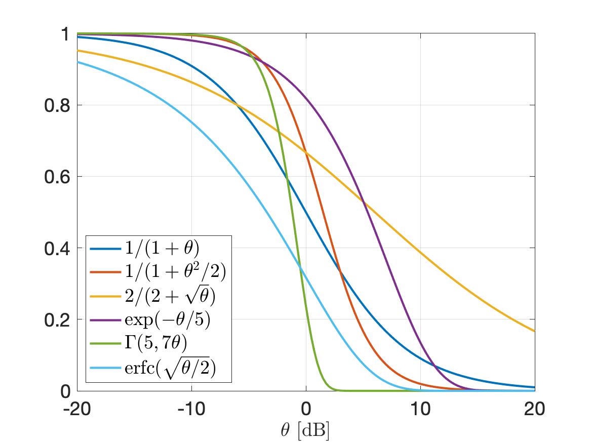
So what is a meaningful graphical model for a wireless network based on which connectivity can be rigorously defined? Let us assume that a transmission succeeds (i.e., a link exists) if the SINR at the receiver exceeds some value θ that is determined based on the coding and modulation schemes. This model incorporates all the physical layer aspects mentioned above and, if made dynamic, channel access and other time-varying aspects.

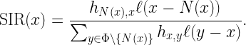
Letting Φ denote the set of node locations (vertices), the SINR-based (geometric) digraph at time k has the directed edge set

$\displaystyle \vec{E}_k=\{(x,y)\in\Phi^2\colon \mathbf{1}({\rm SINR}_{xy}>\theta)\},$

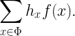
SINR_xy is the SINR at y when it attempts to receive from x at time k. The SINR condition implies that for an edge to form, x is transmitting at time k while y is not (unless y is full-duplex-capable). Then

$\displaystyle G_n\left(\Phi,\bigcup_{k=1}^n \vec{E}_k\right),$

is a directed multigraph (multiple edges are allowed between two vertices) that captures the entire history of successful transmissions in the network up to time n. It may be called the space-time SINR multigraph at time n. Figure 1 shows movie of the evolution of a network with 36 nodes that are transmitting independently with probability 1/4 in each time slot (slotted ALOHA).

Fig. 1. Example of space-time SIR multigraph with θ=3, path loss exponent 4, no noise, and Rayleigh fading. Filled circles indicate transmitters. Edges get thicker each time their link succeeds, and they turn red when bidirectionally is first achieved.

Figure 2 shows a larger network of the same type, with 400 nodes.

Fig. 2. Same as Figure 1 but with 400 nodes.

This graph reveals how many nodes can be reached from a given node within a certain time, or how many other nodes a node can receive a message from. Information in the network propagates along causal paths, i.e., paths where the first link is established before the second before the third, etc. To simplify the identification of such paths, the time index when an edge is established can be added as an edge weight.

Based on this graph, notions of percolation and connectivity can be rigorously defined. For connectivity, a natural definition is that the network is connected if causal paths exist between all pairs of nodes. A fairly general result can be proven without much difficulty: For arbitrary deterministic Φ∈ℝ², ALOHA with transmit probability 0<p<1, a path loss exponent greater than 2, the graph G_∞ is almost surely connected if the (independent) fading variables have infinite support, irrespective of the noise level.

When an analysis for a deterministic set of locations Φ seems hard, randomizing it to a point process may improve the tractability. A good starting point, as usual, is the PPP. For the PPP, one can hope to answer questions such as:

How long does it take on average for a message to propagate from node x to node y (first-passage percolation)? Here x and y are deterministically added to the node set.
Under which condition is the average time for a node to reach any other node infinite? (If this average time is infinite, the node could be declared isolated.)
Is the propagation speed, defined as the time it takes for information to travel from x to y normalized by their distance, zero or positive asymptotically as the distance grows to infinity?

Based on these results, parameters such as the transmit probability can be optimized.

Percentage games

Let us consider a hypothetical situation where the authors of a paper promise the following:

“In the next figure, we compare our Quantum Ultra-Enhanced Superior-Throughput Intelligent Objectively-Novel Adaptive Beamformed Low-Latency Emission (QUESTIONABLE) scheme with the Arbitrarily-Massive Antenna Zero-Innovation Neural Grandiloquence (AMAZING) scheme, which is the best previously known scheme. As the figure shows, the QUESTIONABLE scheme outperforms the AMAZING scheme by 6122% at a threshold of 2 dB.”

They refer to this figure:

Fig. 1: *Fair comparison of our QUESTIONABLE scheme with the AMAZING scheme reported elsewhere. As is clearly apparent, the reliability gain at 2 dB is very high, unquestionably.*

A gain of more than 6,000% sounds, well, amazing. But it also questionable: Is it good practice to state this figure of 6122%? Is it good marketing? Is it acceptable? Should it be discouraged? Is it even unethical?
If claiming 6122% at 2 dB is acceptable, how about a 25119% gain at 10 dB? Here the absolute reliability of AMAZING is 6.3e-9, and that of QUESTIONABLE is 1.60e-6. Not a practical regime, but a more than 25000% gain nonetheless.

Conversely, at -1.5 dB, the improvement is from 0.996 (which is AMAZING) to 0.9999999 (which is QUESTIONABLE). This is a modest 0.4% improvement both in absolute and relative terms. However, focusing on outage instead of reliability, the factor between the two outage probabilities is 62763, or 6,276,267%. So the 0.4% gap becomes a 6M% gap (that’s mega-percent, admittedly an usual combination of a metric prefix with a unit).

Independently of such amazing and questionable transmission schemes, is an improvement from 10% to 13% a 3% improvement or a 30% improvement? Frequently we see such a gain reported as a 30% improvement. Is it fair to use the ratio to measure improvement, or should it be the gap (difference)? Equivalently, should the percentage improvement be measure in percent of the underlying quantity (in which case it is 3%) or in percent of the percentages (in which case it is 30%)? The problem is that terms like “gain”, “increase”, “improvement”, “boost”, “raise” are imprecise as they may refer to differences or ratios.

How about an improvement from 10 dB to 13 dB? Here, most people would agree that the gain is 3 dB. The reason why there is no ambiguity here is that 3 dB is both the difference 13 dB-10 dB and also the ratio of the underlying quantities expressed in dB, 20/10. Thanks to the logarithm in the dB scale, both lead to the same result. With percentages, this is not the case.

The ambiguity also manifests itself when we compare percentages with physical units such as meters or seconds. The difference between 10 m and 13 m is 3 m, and 13 m is 30% longer than 10 m. Percentage gains always measure ratios in this case. But if “meter” is replaced by “percent”, the situation becomes murky. By analogy then the difference between 10% and 13% is 3%, so 13% is 3% more than 10%, in the same way that 13 m is 3 m more than 10 m. But at the same time, 13% is 30% more than 10%, in the same way that 13 m is 30% more than 10 m.

So how do we resolve this? Here are some suggestions:

Always state whether we refer to ratios or difference. For instance, instead of saying “The increase is 30%” say the “increase is a factor of 1.3 or 30%”.
Avoid ambiguity by using fractions instead of percentages. For instance, the difference between 0.1 and 0.13 is 0.03, and the ratio is 1.3.
Avoid aggressive marketing when quantities are in very impractical regimes. For instance, in the example above, advertising huge gains at reliabilities below 1e-5 is not good practice. Conversely, in regimes of interest, such as the high-reliablity regime, it is perfectly acceptable to report a gain of 100 in the outage performance if the outage probability is reduced from 0.01 to 0.0001. (However, talking about 10,000% is not recommended.)
Consider using horizontal distances (gaps) instead of vertical ones. Especially with steep (almost step-like) curves like the one in Fig. 1, the vertical gap strongly depends on where it is measured along the x axis. Conversely, the horizontal gap may be fairly constant. In the case of Fig. 1, the horizontal gap is, in fact, constant. It is exactly 3 dB at all reliabilities. A quasi-constant gap is often observed in SIR distributions (cdfs) of cellular networks when different transmission schemes are compared. The theory behind is explained in this letter (here on IEEE Xplore) and in this paper (here on IEEE Xplore). In this case, the gains are either factors (in linear scale) or gaps (in the dB) scale. This method of reporting gains is the one adopted by the coding theory community – coding gains are reported in dB (horizontally), not as gains in the bit error performance (vertically).

Are users needed in cellular networks?

Let us consider the downlink of a cellular network where base stations form a stationary and ergodic point process Φ and define the SIR at each location x ∈ R² as

$\displaystyle \text{SIR}(x)=\frac{h_{N(x),x}\ell(x-N(x))}{\sum_{y\in\Phi\setminus\{N(x)\}} h_{x,y}\ell(y-x)}.$

Here N(x) is the nucleus of the Voronoi cell that x belongs to, h_x,y is the fading coefficient between x and y, and ℓ is the path loss function. Due to the stationarity of Φ, the SIR statistics do not depend on the location x. In other words, any arbitrary location can be taken to be the typical location that the analysis focuses on.
Example result: If Φ is Poisson, the fading is Rayleigh, and ℓ is a power-law function with exponent 2/δ, it is known that for all x ∈ R²,

$\displaystyle \qquad\qquad\mathbb{P}(\text{SIR}(x)>\theta)=\frac{1}{\,_2F_1(1,-\delta;1-\delta,-\theta)},\qquad\qquad\qquad (1)$

where ₂F₁ is the Gauss hypergeometric function.
Since Φ is ergodic, the probability that the SIR exceeds θ is the fraction of the plane that achieves an SIR of at least θ for all realizations of Φ. This means that the probability (ensemble average) can be replaced by a spatial average over an increasingly large region. Sometimes this probability (or spatial average) is questionably called “coverage probability” (see this post), and the area fraction is termed “covered area fraction”.
It is important to note that results such as (1) do not require any specification of a point process of users. This answers the question in the title: No, users are not necessary in the downlink SIR analysis.

That said, in the literature we observe that in many cases, a point process of users is defined before such downlink SIR results are derived. The reason could be that it may seem overly abstract to consider a cellular network model devoid of any users and view the SIR as a random field on the plane. Specializing the location x to the points of a user point process (assumed independent of Φ), we observe that (1) is the SIR distribution at the typical user for any stationary point process of users. So there is nothing wrong in introducing a point process of users, focus on the typical user, and state a result such as (1). It would, however, be potentially misleading to specify the user point process to be a Poisson process, since the reader may then believe that the result only holds for Poisson distributed users.

There is one caveat when introducing a point process of users to formulate downlink results: The interpretation of the SIR distribution as the fraction of users who achieve SIR>θ in each realization of the user and base station point processes may no longer be correct, even if the two point processes are independent and stationary and ergodic. For instance, consider the case where both are stationary (i.e., randomly translated) lattices of the same intensity. Then, given the point processes, the SIR distribution at each user is the same and depends on the relative shift of the lattices. For example, if a user is very close to its serving base station, then all users are close to their serving base station, and the SIR at all users is likely to exceed θ even when θ is, say, 20 dB. In contrast, if one user is equidistant to two base stations, then all users are, and it is unlikely that the SIR (at any or all of them) exceeds 1. So averaging over the users in one realization cannot yield the same result as averaging over the point processes (ensemble averaging). But doesn’t ergodicity imply that the two results are the same? The answer is yes, it does, but individual ergodicity of the two point processes is not sufficient. Since the SIR depends on both of them jointly, they need to be jointly ergodic. This is the condition that is not met in this example scenario of two lattices.

Physical quantities and scale-free results

Sometimes we read in a paper “the link distance is d meters”. Then, a bit later, “In Fig. 3, we set d=10 m”. Putting the two together, this means that “the link distance is 10 m meters”, which of course isn’t what the authors mean. It is not hard to infer that they mean the distance is 10 m, rather than 10 m². But then why not just say “the link distance is d” from the outset?

Physical quantities are a combination of a numerical value and a unit. If symbols refer to physical quantities, equations are valid irrespective of any metric prefixes used. For example, if the density of a two-dimensional stationary point process is λ, then the mean number of points in a disk of radius r is always λπr². We can express the radius as r=100 m or as r=0.1 km or r=10000 cm, and the density could be λ=0.1 km^-2 or λ=10^-5 m^-2. In contrast, if a symbol only refers to the numerical value of the physical quantity, the underlying unit (and prefix) needs to be specified separately, and the reader needs to keep it in mind. For example, writing λ=10 and r=2 does not tell us anything about the mean number of points in the disk without the units. If the density is said to be λ m^-2 and the radius is said to be r km, then we can infer that there are 40,000,000π points on average in the disk, but if the radius is r m, then there are a mere 40π points.

Separating the numerical values from the units also comes at a loss in flexibility. The advantage of the SI unit system with its metric prefixes is that we can express small and large values conveniently, such as d=5 nm or f=3 THz. Hard-wiring the units by saying “the frequency is f Hz” means that we have to write f=3,000,000,000,000 instead – and expect the reader to memorize that f is expressed in Hz. One may argue that in this case it would be natural to declare that “the frequency is f THz”, but what if much lower frequencies also appear in the paper? A Doppler shift of 10 kHz would become a Doppler shift of f=0.00000001.

This leads to the next problem, which is that some quantities are naturally expressed at a different scale (i.e., with a different metric prefix) than others. Transistor gate lengths are usually expressed in nm, while lengths of fiber optic cables may be expressed in km, and many other lengths and distances fall in between, say wavelengths, antenna spacing, base station height, intervehicular distances etc. Can we expect the readers to keep track of all the base units when we write “the gate length is u nm”, “the wavelength is v cm”, and “the base station height is h m”?

In conclusion, there is really no advantage to this kind of separation. In other words, having mathematical symbols refer to physical quantities rather than just numerical values (while the unit is defined elsewhere) is always preferable.

Now, there are cases, where it makes perfect sense to omit a unit when defining a quantity, say a density or a distance. For example, the normalized notation r=10 or λ=3 is acceptable (usually even preferred) when the normalization reference can be arbitrary. For example, the classical result for the SIR distribution in Poisson bipolar networks (link distance r, path loss exponent 2/δ, Rayleigh fading) is

$\displaystyle F(\theta)=\exp(-c(\delta)\lambda r^2\theta^\delta),$

irrespective of whether r is normalized by 1 m or 1 km – as long as λ is normalized accordingly, i.e., by 1 m^-2 or 1 km^-2). Such scale-free results are particularly elegant, because they show that shrinking or expanding the network does not change the result. They may also indicate that one parameter can be fixed without loss of generality. In this example, what matters is the product λ r², so setting λ=1 or r=1 is sensible to reduce the number of parameters.

One more thing. The conflation of a unit and a noun describing a physical quantity or device has become somewhat popular, unfortunately. It violates rule of proper English composition and also the guidelines for scientific writing as put forth by, for example, IEEE. Let us hope they do not spread further, otherwise we need to get used to THzFrequencies, cmDistances, MsLifetimes, pJConsumptions, km^-2Densities etc. Further, improper capitalization can drastically change the quantities. The gap between a mmLength and a MmLength is 9 orders of magnitude, that between a pASource and a PASource is 27 orders of magnitude, and that between ymGaps and YmGaps is 48 orders of magnitude!

Unmasking distributions with infinite support

When visualizing distributions with infinite support, we face the challenge that they can only be shown partially. Usually we try to judiciously choose the interval of our plot so that the interesting part is revealed, and it is understood that outside that interval the function is essentially zero (for a density) or essentially zero or one (for a cumulative distribution). However, there are two disadvantages to that approach: First, if two distributions are not shown on the same interval, it is hard to compare them. Second, interesting asymptotic behavior in the tails are masked. In many cases, using a linear scale suffers from a third shortcoming: Interesting features may occur on a significantly different scale. Which would require choosing a large interval, but that, in turn, may mask the behavior in some parts.

When plotting distribution of signal-to-interference ratios (SIRs), the standard approach is to use a dB scale. The complementary cumulative distribution (ccdf) is usually interpreted as the success probability of a transmission (in an interference-limited setting). While the dB scale allows for visualization the cccdf over a larger range, it has its own shortcomings: First, it turns the one-sided infinite support [0,∞) into the two-sided infinite support (-∞,∞), which can make selecting a suitable interval harder. Second, it distorts the ccdf, which prevents the viewer from obtaining insight into asymptotic behaviors.

So how can we resolve these issues? It turns out that there is a straightforward solution. It is based on a homeomorphic mapping of [0,∞) to the unit interval [0,1]. This mapping is given by the function T(x)=x/(1+x), and the resulting scale is called MH (Möbius homeomorphic) scale. For comparison, the dB scale has the mapping 10 log₁₀(x). In the figures below, the dummy variable is θ, and we have θ dB=10^θ/10, and θ MH=θ/(1-θ). In the important high-reliability regime θ→0, θ MH ∼ θ, i.e., there is no distortion.
The three figures show 6 ccdfs on a linear, dB, and the MH scale. Clearly, the linear scale plots mask the information about the tail. Some curves go to zero (too) quickly, while the behavior of the yellow one past 100 is completely hidden. The dB scale displays the transitional regime more prominently, but all curves have an inverted S shape, which reduces the discriminative power of these plots. In particular, for small θ, they all become flat. For example, the blue (Pareto) and the cyan (Lévy) curve look similar in the dB scale, but with some shift. The MH scale, however, reveals that the asymptotic behavior on both ends is, in fact, quite different. Also, the red (another Pareto distribution) and green (gamma) curve look fairly similar in the dB scale, while the MH scale emphasizes the difference between the two. Generally, the MH plots enhance the differences because the slopes at 0 and at 1 can assume any value, while the slopes in the dB plots always approach 0 – assuming the range is chosen wide enough.

In summary, the MH scale has the following advantages:

There is a single finite interval that reveals the complete distribution. There is never a question of what interval to choose, and nothing remains hidden.
The asymptotic behaviors are clearly visible. In comparison, on the dB scale, the behavior near 0 and towards infinity is always obscured.
In the case of SIRs, the MH scale has the additional interpretation as visualizing the distribution of the signal fraction S/(S+I) (SF) on a linear scale: If F(θ) is the ccdf of the SIR S/I, then F(T(θ)) is the ccdf of the SF.

The MH mapping and its application to SIRs and signal fractions was first introduced in the invited paper M. Haenggi, “SIR Analysis via Signal Fractions”, IEEE Communications Letters, vol. 24, pp. 1358-1362, July 2020.

decibels — Figure 2. Same ccdfs on a dB scale (corresponding to [0.01,100] in the linear scale).

mh_scale — Figure 3. Same ccdfs on the MH scale.

Over-indexing and undefined expressions

Reading the literature, we often encounter sums of the form

$\displaystyle\sum_{x_k\in\Phi} f(x_k)$

for a point process Φ. This is an instance of what may be called “over-indexing”, since the subscript k is clearly not needed. It makes the notation unnecessarily cumbersome, but there is nothing mathematically wrong with it. If it is tacitly assumed that using a dummy variable of the form x_k somehow defines k, problems arise. For instance, what exactly is meant by this formula?

$\displaystyle\sum_{x_k\in\Phi} f(k)$

To make this concrete, let us focus on this simple form:

$\displaystyle\sum_{n_k\in\{1,2,3\}} k^2$

What is the result? It is not 14 but undefined, since k is undefined. This problem occurs fairly frequently in the form

$\displaystyle\sum_{x_k\in\Phi} h(k)f(x_k)\qquad\text{or}\qquad \sum_{x_k\in\Phi} h_k f(x_k)$

where h(k) is used to denotes a fading random variable indexed by some (undefined) k and f is a path loss function. What is meant is usually

$\displaystyle\sum_{k\in\mathbb{N}} h(k)f(x_k),\quad\text{where }\Phi=\{x_1,x_2,\ldots\}.$

Alternatively,

$\displaystyle\sum_{x\in\Phi} h_x f(x).$

Here the fading random variables are indexed by the points, i.e., they can be interpreted as marks associated with the points. This is the form I personally prefer, for it does not require a particular way of indexing the points and it is more compact.

On the typical point

The concept of the typical point is important in point process theory. In the wireless context, it is often concretized to the typical user, typical receiver, typical vehicle, etc. The typical point is an abstraction in the sense that it is not a point that is selected in any deterministic fashion from the point process, neither is it an arbitrary point. Also, speaking of “a typical point” is misleading, since it suggests that there exist a number of such typical points in the process (or perhaps even in a realization thereof), and we can choose one of them to “obtain a typical point”. This does not work – there is nothing “typical” about a point selected in a deterministic fashion, let alone an arbitrary point.
That said, if the total number of points is finite, we can, loosely speaking, argue that the typical point is obtained by choosing one of the points uniformly at random. Even this is not trivial since picking a point in a single realization of the point process does generally not produce the desired result, for example of the point process is not ergodic. Many realizations need to be considered, but then the question arises how exactly to pick a point uniformly from many realizations. If the number of points is infinite, any attempt of picking a point uniformly at random is bound to fail because there is no way to select a point uniformly from infinitely many, in much the same way that we cannot select an integer uniformly at random.

So how do we arrive at the typical point? If the point process is stationary and ergodic, we can generate the statistics of the typical point by averaging those of each individual point in a single realization, observed in an increasingly large observation window. This leads to the interpretation of the typical point as a kind of “average point”. Similarly, we may find that the “typical American male” weighs 89.76593 kg, which does not imply that there exists an individual with that exact weight but means that if we weighed every(male)body or a large representative sample, we would obtain that average weight. For general (stationary) point processes, we obtain the typical point by conditioning on a point to exist at a certain location, usually the origin o. Upon averaging over the point process (while holding on to this point at the origin), that point becomes the typical point. The distribution of this conditioned point process is the Palm distribution. In the case of the Poisson process, conditioning on a point at o is the same as adding a point at o. This equivalence is called Slivnyak’s theorem.

In the non-stationary case, the typical point at location x may have different statistical properties than the typical point at another location y. As a result, there exist Palm measures (or distributions) for each location in the support of the point process. In this case, the formal definition of the Palm measure is given by the Radon-Nikodym derivative (with respect to the intensity measure) of the Campbell measure. In the Poisson case, Slivnyak’s theorem still applies.