What do you call a stationary point process of intensity 0?


Pointless.
A blog on stochastic geometry
Month: December 2020
What do you call a stationary point process of intensity 0?
Pointless.
The analysis of cellular networks usually focuses on the typical user in the downlink and the typical base station (or, equivalently, the typical cell) in the uplink. It is important that if base station and user point processes are independent, the two notions of “typical” are not compatible – the typical user’s cell is statistically different from the typical cell. The difference is caused by the effect of size-biased sampling. The typical user’s performance corresponds to that of the average of all users, and there are more users in larger cells. Since a user model is not needed in the downlink as explained in this post, we can equivalently say that an arbitrary location is more likely to fall in a larger cell than a smaller cell.
The typical user’s cell, the so-called 0-cell, is the cell containing the origin, i.e., it is obtained by cell area-biased sampling, which gives larger cells more weight. As a result, the 0-cell is larger on average than the typical cell, which is the cell of the base station conditioned to be at the origin. The statistical properties of the typical cell correspond to the averages of all cells.
Such size-biased sampling is not restricted to cellular networks or stochastic geometry. If we throw a dart blindly on a world map until we hit land, the country we hit is quite likely to be a big one. In fact, there is a 50% chance that the dart lands on one of the 10 largest countries. Similarly, the typical country has 40 M inhabitants on average, but the typical person is likely to live in a country with more than 100 M people. The typical dollar is quite likely owned by a wealthy person, while the typical person is probably not rich. The typical human hair is likely to grow on a person with full hair, while the typical person has a 5-10% chance of being bald. The typical animal leg has a decent chance of belonging to a millipede or centipede, while the typical animal is very unlikely to have more than six feet.
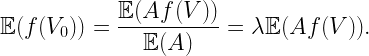
Coming back to cellular networks, let us focus on a concrete example that is fully tractable in terms of the cell area distributions. Consider the lattice with holes shows in Fig. 1 below, obtained from a square lattice of density 1 by removing the four nearest neighbors of each 16th point. It is periodic with period 4 in both directions, its density is λ=3/4, and it has four different types of cells, with three different areas, 1, 3/2, and 2.
The typical cell has area 1 with probability 5/12, area 3/2 with probability 1/2, and area 2 with probability 1/12. The mean area follows as E(A)=5/12+1/2 3/2+1/12 2=4/3, which corresponds to 1/λ.
Now assume a stationary square lattice of density 1 as the user point process. Then the cells of area 1 always contain 1 user and those of area 2 always contain 2 users. Those of area 3/2 have 1 user or 2 users, each with probability 1/2. Deconditioning on the cell areas, we obtain the distribution of the number of users U in the typical cell as P(U=1)=2/3 and P(U=2)=1/3, for a mean number of users E(U)=4/3, which equals the mean area times the user density (chosen to be 1 here).
How about the typical user’s cell? This is where the size bias plays a role. The distribution of the area A0 of the 0-cell is P(A0=1)=5/16, P(A0=3/2)=9/16, and P(A0=2)=1/8. These are the fractions of the plane covered by cells of areas 1, 3/2, and 2. The mean area is E(A0)=45/32, which is about 5.5% bigger than the mean area of the typical cell. The number of users U0 in the 0-cell is distributed as P(U0=1)=5/16+1/2 9/16=19/32, P(U0=2)=1/2 9/16+1/8=13/32, resulting in a mean of E(U0)=45/32, which is the user density times the mean area. The mean also follows from the general formula
where V is the typical cell, V0 the 0-cell, and f is a non-negative function on compact sets. Applied to our setting, where f(V) is the number of users in V, we obtain
Since the user density is 1, this is also the mean area of A0. For the number of sides S, we have E(S)=19/4, but E(S0)=155/32, which is bigger by 3/32.
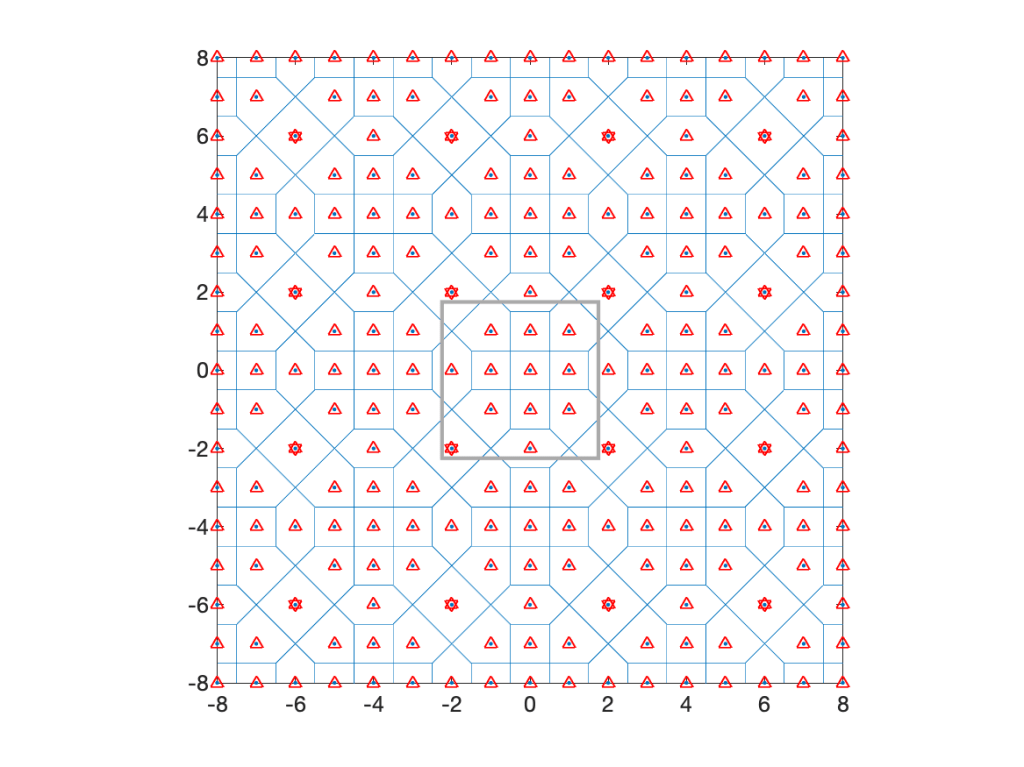
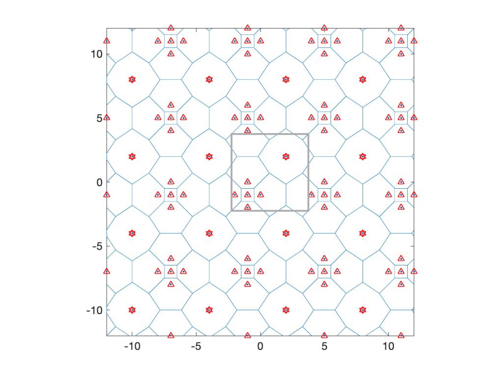
At the end of this post are three more examples of similarly constructed lattices. In each case, the points within a certain distance of a sub-lattice are removed.
So the typical user is not served by the typical base station, and the typical base station does not serve the typical user. One way to reconcile the two is to define a user point process where a fixed number of users, say one, is placed uniformly at random in each cell. Such a user process is of course no longer independent of the base station process.
For Poisson distributed base stations, the 0-cell is 28% larger than the typical cell. Its mean number of sides is 6.41, whereas the typical cell has 6 sides on average. Hence the 0-cell is not just an enlarged version of the typical cell but also has a different shape. Accordingly, the distance from the nucleus of the typical cell to a random point in the cell is not Rayleigh distributed as it is in the 0-cell. Also, if users form a PPP of density 1, the typical user’s cell has 1+1.28/λ users on average (there is one extra user due to the conditioning of a user to be at the origin), while the typical cell only has a mean of 1/λ users.
Size-biased sampling is important in other wireless networks as well. If a vehicular network is modeled by placing one-dimensional Poisson point processes (cars) on line segments (streets) of independent random length (which is a Cox process supported on line segments), then the typical vehicle’s street length distribution fL0 is different from the length distribution f_L of the streets. By length-biased sampling, the two are related as
For example, if L is exponential with mean 1, then L0 is gamma distributed with mean 2. The same situation arises in the interarrival intervals of a one-dimensional PPP (of density 1). The typical such interval is exponential with mean 1, but the interval containing the origin (or any other deterministic time instant) has a mean length of 2. This is sometimes referred to as the waiting time paradox, although there is nothing paradoxical about it – it is just size-biased sampling.
Lastly, as promised, here are three more examples of lattices with increasingly large holes.


In recent years, many research efforts were dedicated towards modeling and analyzing denser and denser wireless networks, in terms of the number of devices per km2 or m2. The terminology used ranges from “ultradense” to “hyperdense”, “massively dense”, and “extremely dense”.
IEEE Xplore lists more than 500 journal papers on “ultradense” networks, 25 on “hyperdense” networks (generally published more recently than the ultradense ones), and about 90 on “extremely dense” networks. There even exist 15 on “massively dense” networks. The natural question is how they are ordered. Is “ultradense” denser than “hyperdense” or vice versa? How does “extremely dense” fit in? Are there clear definitions what the different levels of densities mean? And what term do we use when networks get even denser?
Perhaps we can learn something from the terminology used for frequency bands. There is “high frequency” (HF), “very high frequency” (VHF), “ultrahigh frequency” (UHF), followed by “super high frequency” (SHF), “extremely high frequency” (EHF), and “tremendously high frequency” (THF). The first five each span an order of magnitude in frequency (or wavelength), while the last ones spans two order of magnitude, from 300 GHz to 30 THz.
So how about we follow that approach and classify network density levels as follows:
HD: 1-10 km-2
VHD: 10-100 km-2
UHD: 100-1’000 km-2
SHD: 1’000-10’000 km-2
EHD: 10’000-100’000 km-2
THD: 0.1-10 m-2
So, who will be the first to write a paper on tremendously dense networks?
What comes after THD? Not unexpectedly, there is a mathematical answer to that question. A dense set has a well-defined meaning. So in the super tremendously extreme case, we can just say that the devices are dense on the plane, without further qualification. This is achieved, for instance, by placing a device at each location with rational x and y coordinates. This is a dense network model, and almost surely there is no denser one.
The attributes “tractable”, “closed-form”, and “exact” are frequently used to describe analytical results and, in the case of “tractable”, also models. At the time of writing, IEEE Xplore lists 4540 journal articles with “closed-form” and “wireless” in their meta data, 650 with “tractable” and “wireless”, and 220 with “closed-form”, “wireless” and “stochastic geometry”.
Among the three adjectives, only for “exact” there is general consensus what is means exactly. For “closed-form”, mathematicians have a clear definition: The expression can only consist of finite sums and products, division, roots, exponentials, logarithms, trigonometric and hyperbolic functions and their inverses. Many authors are less strict, using the term also for expressions involving general transcendent functions or infinite sums and products. Lastly, the use of “tractable” varies widely. There are “tractable results”, “tractable models”, “tractable analyses”, and “tractable frameworks”.
“Tractable” is defined by Merriam-Webster as “easily handled, managed, or wrought”, by the Google Dictionary as “easy to deal with”, and by the Cambridge Dictionary as “easily dealt with, controlled, or persuaded”. Wikipedia refers to the mathematical use of the term: “ease of obtaining a mathematical solution such as a closed-form expression”. These definitions are too vague to clearly distinguish a “tractable model” from a “non-tractable” one, since “easy” can mean very different things to different people.
We also find combinations of the terms; in the literature, there are “tractable closed-form expressions” and even “highly accurate simple closed-form approximations”. But shouldn’t all “closed-form” expressions qualify as “tractable”? And aren’t they also “simple”, or are there complicated “closed-form” expressions?
It would be helpful to find an agreement in our community what qualifies as “closed-form”. Here is a proposal:
Thus equipped, we could try to define what a “tractable model” is. For instance, we could declare a model “tractable” if it allows the derivation of at least one non-trivial exact closed-form result for the metric of interest. This way, the SIR distribution in the Poisson bipolar network with ALOHA, Rayleigh fading, and power-law path loss is tractable because the expression only involves an exponential and a trigonometric function. The SIR in the downlink Poisson cellular with Rayleigh fading and path loss exponent 4 is also tractable; its expression includes only square roots and an arctangent. In contrast, the SIR in the uplink Poisson cellular network is not tractable, irrespective of the user point process model.
A result could be termed “tractable” if the typical educated reader can tell how the expression behaves as a function of its parameters.
Going a step further, it may make sense to be more formal and introduce categories for the sharpness of a result, such as these:
A1: closed-form exact
A2: weakly closed-form exact
A3: general exact
B1: closed-form bound
B2: weakly closed-form bound
B3: general bound
C1: closed-form approximation
C2: weakly closed-form approximation
C3: general approximation
Alternatively, we could use A+, A, A-, B+, etc., inspired by the letter grading system used in the USA. We could even calculate a grade point average (GPA) of a set of results, based on the standard letter grade-to-numerical grade conversion.
Such classification allows a non-binary quantification of “tractability” of a model. If the model permits the derivation of an A1 result, it is fully “tractable”. If it only allows C3 results, it is not “tractable”. If we can obtain, say, an A3, a B2, and a C1 result, it is 50% “tractable” or “semi-tractable”. Such a sliding scale instead of a black-and-white categorization would reflect the vagueness of the general definition of the term but put it on a more solid quantitative basis. Subcategories for asymptotic results or “order-of” results could be added.
This way, we can pave the way towards the development of a tractable framework for tractability.