November 2021 – Stogblog by M. Haenggi

Naturally the locations of wireless transceivers are modeled as a point process on the plane or perhaps in the three-dimensional space. However, key quantities that determine the performance of a network do not directly nor exclusively depend on the locations but on the received powers. For instance, a typical SIR expression (at the origin) looks like

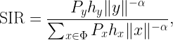
$\displaystyle {\rm SIR}=\frac{P_y h_y \|y\|^{-\alpha}}{\sum_{x\in\Phi} P_x h_x \|x\|^{-\alpha}},$

where y is the location of the intended transmitter and Φ is the point process of interferers. P_x and h_x are the transmit powers and fading coefficients of x, respectively. It is apparent that what matters are the distances raised to some power, not the locations themselves. So instead of working with Φ⊂ℝ², we can focus on the one-dimensional process

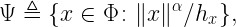
$\displaystyle \Psi\triangleq\{x\in\Phi\colon \|x\|^{\alpha}/h_x\},$

called the path loss point process (PLPP) (with fading). The reason why the positive exponent α is preferred over -α is that otherwise the resulting point process is no longer locally finite (assuming Φ is stationary) since infinitely many points would fall in the interval [0,ε] for any ε>0. Transmit power levels could be included as displacements, either deterministically or randomly.

Path loss processes are particularly useful when Φ is a PPP. By the mapping and displacement theorems, the PLPPs are also PPPs whose intensity function is easy to calculate. For a stationary PPP Φ of intensity λ and iid fading, the intensity function of Ψ is

$\displaystyle \mu(r)=\pi\lambda\delta r^{\delta-1}\mathbb{E}(h^\delta),\quad r\geq 0, \delta\triangleq2/\alpha.$

where h is a generic fading random variable. If h has mean 1, then for δ<1, which is necessary to keep the interference finite, 𝔼(h^δ)<1 from Jensen’s inequality, hence the effect of fading is a reduction of the intensity function by a fixed factor.

As an immediate application we observe that fading reduces the expected number of connected nodes, defined as those whose received power is above a certain threshold, by the δ-th moment of the fading coefficients.

More importantly, PLPPs lead to two key insights for Poisson cellular networks. Let us assume the elements of Ψ are ordered and denoted as ξ₁<ξ₂<… . Then the SIR with instantaneously-strongest base station association (ISBA) is

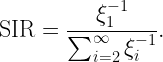
$\displaystyle {\rm SIR}=\frac{\xi_1^{-1}}{\sum_{i=2}^\infty \xi_i^{-1}}.$

First, it is not hard to show that for ISBA with Rayleigh fading, the SIR distribution does not depend on the density of the underlying PPP. But since the effect of fading is but a scaling of the density, it follows that the SIR distribution does not depend on the fading statistics, either. In particular, the result for Rayleigh fading also applies to the non-fading case (where ISBA corresponds to nearest-base station association, NBA), which is often hard to analyze in stochastic geometry models.

Second, the intensity function of the PLPP also shows that the SIR performance of the heterogeneous independent Poisson (HIP) model is the same as that of the simple PPP model. The HIP model consists of an arbitrary number n of tiers of base stations, each modeled as an independent PPP of arbitrary densities λ_k and transmitting at arbitrary (deterministic) power levels P_k. The point process of inverse received powers (i.e., the PLPP with transmit powers included) from tier k has intensity

$\displaystyle \mu_k(r)=\pi\lambda_k\delta r^{\delta-1}\mathbb{E}(h^\delta)P_k^\delta,\quad r\geq 0.$

Since the superposition of n PPPs is again a PPP, the overall intensity is just the sum of the μ_k, which is still proportional to r^δ-1. This shows that the SIR performance (with ISBA or NBA) of any HIP model is the same as that of just a single PPP.

For further reading, please refer to A Geometric Interpretation of Fading in Wireless Networks: Theory and Applications and The Performance of Successive Interference Cancellation in Random Wireless Networks.