Tag: Poisson point process

Meta visualization

In this post we contrast the meta distribution of the SIR with the standard SIR distribution. The model is the standard downlink Poisson cellular network with Rayleigh fading and path loss exponent 4. The base station density is 1, and the users form a square lattice of density 5. Hence there are 5 users per cell on average.

Fig. 1: *The setup. Base stations are red crosses, and users are blue circles. They are served by the nearest base station. Cell boundaries are dashed.*

We assume the base stations transmit to the users in their cell at a rate such that the messages can be decoded if an SIR of θ =-3 dB is achieved. If the user succeeds in decoding, it is marked with a green square, otherwise red. We let this process run over many time slots, as shown next.

Fig. 2: *Transmission success (green) and failure (red) at each user over 100 time slots.*

The SIR meta distribution captures the per-user statistics, obtained by averaging over the fading, i.e., over time. In the next figure, the per-user reliabilities are illustrated using a color map from pure red (0% success) to pure green (100% success).

Fig. 3: *Per-user reliabilities, obtained by averaging over fading. These are captured by the SIR meta distribution*. Near the top left is a user that almost never succeeds since it is equidistant to three base stations.

The SIR meta distribution provides the fractions of users that are above (or below) a certain reliability threshold. For instance, the fraction of users that are at least dark green in the above figure.

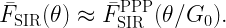
In contrast, the standard SIR distribution, sometimes misleadingly called “coverage probability”, is just a single number, namely the average reliability, which is close to 70% in this scenario (see, e.g., Eqn. (1) in this post). Since it is obtained by averaging concurrently over fading and point process, the underlying network structure is lost, and the only information obtained is the average of the colors in Fig. 3:

Fig. 4: *The standard SIR distribution only reveals the overall reliability of 70%.*

The 70% reliability is that of the typical user (or typical location), which does not correspond to any user in our network realization. Instead, it is an abstract user whose statistics correspond to the average of all users.

Acknowledgment: The help of my Ph.D. student Xinyun Wang in writing the Matlab program for this post is greatly appreciated.

Realistic communication

Today’s blog is about realistic communication, i.e., what kind of performance can realistically be expected of a wireless network. To get started, let’s have a look at an excerpt from a recent workshop description:

“Future wireless networks will have to support many innovative vertical services, each with its own specific requirements, e.g.

End-to-end latency of 1 ns and reliability higher than 99.999% for URLLCs.
Terminal densities of 1 million of terminals per square kilometer for massive IoT applications.
Per-user data-rate of the order of Terabit/s for broadband applications.”

Let’s break this down, bullet by bullet.

First bullet: In 1 ns, light travels 30 cm in free space. So “end-to-end” here would mean a distance of at most 10 cm, to leave some fraction of a nanosecond for encoding, transmission, and decoding. But what useful wireless service is there where transceivers are within at most 10 cm? Next, a packet loss rate of 10^-5 means that the spectral efficiency must be very low. Together with a latency constraint of 1 ns, ultrahigh bandwidths must be used, which, in turn, makes the design of circuitry and antenna arrays extremely challenging. At least the channel can be expected to be benign (line-of-sight).

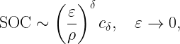
Where does stochastic geometry come in? Assuming that these ultrashort links live in a network and not in isolation, interference will play a role. Let us consider a Poisson bipolar network with normalized link distance 1, a path loss exponent α and Rayleigh fading. What is the maximum density of links that can be supported that have an outage of at most ε? This quantity is known as the spatial outage capacity (SOC). For small ε, which is our regime of interest here, we have

$\displaystyle\text{SOC}\sim\left(\frac{\varepsilon}{\rho}\right)^\delta c_\delta,\quad \varepsilon\to 0,$

where δ=2/α and c_δ is a constant that only depends on the path loss exponent 2/δ. ρ is the spectral efficiency (in bits/s/Hz or bps/Hz). This shows the fundamental tradeoff between outage and spectral efficiency: Reducing the outage by a factor of 10 reduces the rate of transmission by the same factor if the same link density is to be maintained. Compared to a more standard outage constraint of 5%, this means that the rate must be reduced by a factor 5,000 to accommodate the 99.999% reliability requirement. Now, say we have 0.5 ns for the transmission of a message of 50 bits, the rate is 100 Gbps. Assuming a very generous spectral efficiency of 100 bps/Hz for a system operating at 5% outage, this means that 100 Gbps must be achieved at a spectral efficiency of a mere 0.02 bps/Hz. So we would need 5 THz of bandwidth to communicate a few dozen bits over 10 cm.
Even relaxing the latency constraint to 1 μs still requires 5 GHz of bandwidth.

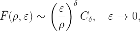
In cellular networks, the outage-rate relationship is governed by a very similar tradeoff.
For any stationary point process of base stations and Rayleigh fading, the SIR meta distribution asymptotically has the form

$\displaystyle \bar F(\rho,\varepsilon)\sim\left(\frac{\varepsilon}{\rho}\right)^\delta C_\delta,\quad \varepsilon\to 0,$

where C_δ again depends only on the path loss exponent. This is the fraction of users who achieve a spectral efficiency of ρ with an outage less than ε, remarkably similar to the bipolar result. To keep this fraction fixed at, say, 95%, again the spectral efficiency needs to be reduced in proportion to a reduction of the outage constraint ε.

Second bullet: Per the classification and nomenclature in a dense debate, this density falls squarely in the tremendously dense class, above super-high density and extremely high density. So what do the anticipated 100 devices in an average home or 10,000 devices in an average parking lot do? What kind of messages are they exchanging or reporting to a hub? How often? What limits the performance? These devices are often said to be “connected“, without any specification what that means. Only once this is clarified, a discussion can ensue whether such tremendous densities are realistic.

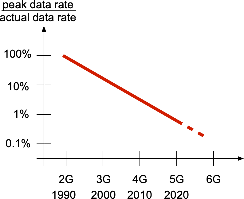
Third bullet: Terabit-per-second (Tbps) rates require at least 10 GHz of spectrum, optimistically. 5G in its most ambitious configuration, ignoring interference, has a spectral efficiency of about 50 bps/Hz, and, barring any revolutionary breakthrough, more than 100 bps/Hz does not appear feasible in the next decade. Similarly, handling a signal 10 GHz wide would be an order of magnitude beyond what is currently possible. Plus such large junks of spectrum are not even available at 60 GHz (the current mm-wave bands). At 100 GHz and above, link distances are even more limited and more strongly subject to blockages, and analog beamforming circuitry becomes much more challenging and power-hungry. Most importantly, though, peak rates are hardly achieved in reality. In the 5G standard, the user experienced data rate (the rate of the 5-th percentile user) is a mere 1% of the peak rate, and this fraction has steadily decreased over the cellular generations:

So even if 1 Tbps peak rates became a reality, users would likely experience between 1 Gbps to at most 10 Gbps – assuming their location is covered, which may vary over short spatial scales. Such user percentile performance can be analyzed using meta distributions.

In conclusion, while setting ambitious goals may trigger technological advances, it is important to be realistic of what is achievable and what performance the user actually experiences. For example, instead of focusing on 1 Tbps peak rates, we could focus on delivering 1 Gbps to 95% of the users, which may still be very challenging but probably achievable and more rewarding to the user. And speaking of billions of “connected devices” is just marketing unless it is clearly defined what being connected means.

For more information on the two analytical results above, please see this paper (Corollary 1) and this paper (Theorem 3).

Signal-to-interference, reversed

Interference is the key performance-limiting factor in wireless networks. Due to the many unknown parts in a large network (transceiver locations, activity patterns, transmit power levels, fading), it is naturally modeled as a random variable, and the (only) theoretical tool to characterize its distribution is stochastic geometry. Accordingly, many stochastic geometry-based works focus on interference characterization, and some closed-form expressions have been obtained in the Poisson case.

If the path loss law exhibits a singularity at 0, such as the popular power-law r^-α, the interference (power) may not have a finite mean if an interferer can be arbitrarily close to the receiver. For instance, if the interferers form an arbitrary stationary point process, the mean interference (at an arbitrary fixed location) is infinite irrespective of the path loss exponent. If α≤2, the interference is infinite in an almost sure sense.

This triggered questions about the validity of the singular path loss law and prompted some to argue that a bounded (capped) path loss law should be used, with α>2, to avoid such divergence of the mean. Of course the singular path loss law becomes unrealistic at some small distance, but is it really necessary to use a more complicated model that introduces a characteristic distance and destroys the elegant scale-free property of the singular (homogeneous) law?

The relevant question is to which extent the performance characterization of the wireless network suffers when using the singular model.

First, for practical densities, there are very few realizations where an interferer is within the near-field, and if it is, the link will be in outage irrespective of whether a bounded or singular model is used. This is because the performance is determined by the SIR, where the interference is in the denominator. Hence whether the interference is merely large or almost infinite makes no difference – for any reasonable threshold, the SIR will be too small for communication.
Second, there is nothing wrong with a distribution with infinite mean. While standard undergraduate and graduate-level courses rarely discuss such distributions, they are quite natural to handle and pose no significant extra difficulty.

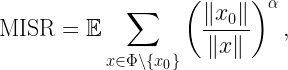
That said, there is a quantity that is very useful when it has a finite mean: the interference-to-(average)-signal ratio ISR, defined as

$\displaystyle {\rm ISR}=\frac{\sum_{x\in\Phi\setminus\{x_0\}} h_x \|x\|^{-\alpha}}{\|x_0\|^{-\alpha}},$

where x₀ is the desired transmitter and the other points of Φ are interferers. The h_x are the fading random variables (assumed to have mean 1), only present in the numerator (interference), since the signal power here is averaged over the fading.
Taking the expectation of the ISR eliminates the fading, and we arrive at the mean ISR

$\displaystyle {\rm MISR}=\mathbb{E} \sum_{x\in\Phi\setminus\{x_0\}}\left(\frac{\|x_0\|}{\|x\|}\right)^{\alpha},$

which only depends on the network geometry. It follows that the SIR distribution is

$\displaystyle \mathbb{P}({\rm SIR}<\theta)=\mathbb{P}(h<\theta\, {\rm ISR})=\mathbb{E} F_h(\theta\,{\rm ISR}),$

where h is a generic fading random variable. If h is exponential (Rayleigh fading) and the MISR is finite,

$\displaystyle F_h(x)\sim x\qquad\Longrightarrow\qquad \mathbb{P}({\rm SIR}<\theta)\sim \theta\,{\rm MISR}.$

Hence for small θ, the outage probability is proportional to θ with proportionality factor MISR. This simple fact becomes powerful in conjunction with the observation that in cellular networks, the SIR distributions (in dB) are essentially just shifted versions of the basic SIR distribution of the PPP (and of each other).

Figure 1: Examples for SIR distributions in cellular networks that are essentially shifted versions of each other.

In Fig. 1, the blue curve is the standard SIR ccdf of the Poisson cellular network, the red one is that of the triangular lattice, which has the same shape but shifted by about 3 dB, with very little dependence on the path loss exponent. The other two curves may be obtained using base station silencing and cooperation, for instance. Since the shift is almost constant, it can be determined by calculating the ratios of the MISRs of the different deployments or schemes. The asymptotic gain relative to the standard Poisson network (as θ→0) is

$\displaystyle G_0=\frac{\rm MISR_{PPP}}{{\rm MISR}},\quad \text{where }\; {\rm MISR_{PPP}}=\frac{2}{\alpha-2},\quad \alpha>2,$

The MISR in this expression is the MISR for an alternative deployment or architecture. The MISR for the PPP is not hard to calculate. Extrapolating to the entire distribution by applying the gain everywhere, we have

$\displaystyle \bar F_{\rm SIR}(\theta) \approx \bar F_{\rm SIR}^{\rm PPP}(\theta/G_0).$

This approach of shifting a baseline SIR distribution was proposed here and here. It is surprisingly accurate (as long as the diversity order of the transmission scheme is unchanged), and it can be extended to other types of fading. Details can be found here.

Hence there are good reasons to focus on the reversed SIR, i.e., the ISR.

Path loss point processes

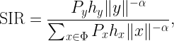
Naturally the locations of wireless transceivers are modeled as a point process on the plane or perhaps in the three-dimensional space. However, key quantities that determine the performance of a network do not directly nor exclusively depend on the locations but on the received powers. For instance, a typical SIR expression (at the origin) looks like

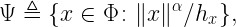
$\displaystyle {\rm SIR}=\frac{P_y h_y \|y\|^{-\alpha}}{\sum_{x\in\Phi} P_x h_x \|x\|^{-\alpha}},$

where y is the location of the intended transmitter and Φ is the point process of interferers. P_x and h_x are the transmit powers and fading coefficients of x, respectively. It is apparent that what matters are the distances raised to some power, not the locations themselves. So instead of working with Φ⊂ℝ², we can focus on the one-dimensional process

$\displaystyle \Psi\triangleq\{x\in\Phi\colon \|x\|^{\alpha}/h_x\},$

called the path loss point process (PLPP) (with fading). The reason why the positive exponent α is preferred over -α is that otherwise the resulting point process is no longer locally finite (assuming Φ is stationary) since infinitely many points would fall in the interval [0,ε] for any ε>0. Transmit power levels could be included as displacements, either deterministically or randomly.

Path loss processes are particularly useful when Φ is a PPP. By the mapping and displacement theorems, the PLPPs are also PPPs whose intensity function is easy to calculate. For a stationary PPP Φ of intensity λ and iid fading, the intensity function of Ψ is

$\displaystyle \mu(r)=\pi\lambda\delta r^{\delta-1}\mathbb{E}(h^\delta),\quad r\geq 0, \delta\triangleq2/\alpha.$

where h is a generic fading random variable. If h has mean 1, then for δ<1, which is necessary to keep the interference finite, 𝔼(h^δ)<1 from Jensen’s inequality, hence the effect of fading is a reduction of the intensity function by a fixed factor.

As an immediate application we observe that fading reduces the expected number of connected nodes, defined as those whose received power is above a certain threshold, by the δ-th moment of the fading coefficients.

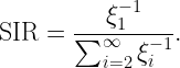
More importantly, PLPPs lead to two key insights for Poisson cellular networks. Let us assume the elements of Ψ are ordered and denoted as ξ₁<ξ₂<… . Then the SIR with instantaneously-strongest base station association (ISBA) is

$\displaystyle {\rm SIR}=\frac{\xi_1^{-1}}{\sum_{i=2}^\infty \xi_i^{-1}}.$

First, it is not hard to show that for ISBA with Rayleigh fading, the SIR distribution does not depend on the density of the underlying PPP. But since the effect of fading is but a scaling of the density, it follows that the SIR distribution does not depend on the fading statistics, either. In particular, the result for Rayleigh fading also applies to the non-fading case (where ISBA corresponds to nearest-base station association, NBA), which is often hard to analyze in stochastic geometry models.

Second, the intensity function of the PLPP also shows that the SIR performance of the heterogeneous independent Poisson (HIP) model is the same as that of the simple PPP model. The HIP model consists of an arbitrary number n of tiers of base stations, each modeled as an independent PPP of arbitrary densities λ_k and transmitting at arbitrary (deterministic) power levels P_k. The point process of inverse received powers (i.e., the PLPP with transmit powers included) from tier k has intensity

$\displaystyle \mu_k(r)=\pi\lambda_k\delta r^{\delta-1}\mathbb{E}(h^\delta)P_k^\delta,\quad r\geq 0.$

Since the superposition of n PPPs is again a PPP, the overall intensity is just the sum of the μ_k, which is still proportional to r^δ-1. This shows that the SIR performance (with ISBA or NBA) of any HIP model is the same as that of just a single PPP.

For further reading, please refer to A Geometric Interpretation of Fading in Wireless Networks: Theory and Applications and The Performance of Successive Interference Cancellation in Random Wireless Networks.

The transdimensional approach

In vehicular networks, transceivers are inherently confined to a subset of the two-dimensional Euclidean space. This subset is the street system where cars are allowed to move. Accordingly, stochastic geometry models for vehicular networks usually consist of two components: A set of streets and a set of point processes, one for each street, representing the vehicles. The most popular model is the Poisson line process (PLP) for the streets, combined with one-dimensional PPPs of vehicles on each line (street).

This PLP-PPP model does not have T-junctions, only intersections. Accordingly, all vehicles are of order 2 or 4, per the taxonomy introduced here. The order is determined by the number of directions in which a vehicle can move.

The PLP-PPP is a Cox process due to the independent one-dim. PPPs, and the underlying street system determining the intensity measure (the line process) is also based on the PPP. Consequently, the PLP-PPP inherits a certain level of tractability from the PPP, in the sense that exact expressions can be derived for some quantities of interest. In particular, the SIR distribution (complementary cumulative distribution function, ccdf) at the typical vehicle for a transmitter at a fixed distance can be derived without difficulty. However, the expression requires the evaluation of two nested improper integrals. While such a result certainly has its value, it does not give direct insight how the resulting SIR distribution depends on the network parameters. Also, other metrics that depend on the SIR often require further integration, most importantly the SIR meta distribution, which is calculated from the higher moments of the conditional SIR ccdf (given the point process).

This raises the question whether it is possible to find a closed-form result that is much more quickly evaluated and provides a tight approximation. Simply replacing the PLP-PPP by a two-dimensional PPP produces poor results, especially in the high-reliability regime (where the SIR ccdf is near 1). Similarly, considering only the one street that the typical vehicle lies on (i.e., using only a one-dimensional PPP) ignores all the interference from the vehicles on the other streets, which strongly affects the tail of the distribution.

How about a combination of the two – a superposition of a one-dimensional PPP for the typical vehicle’s street and a two-dimensional PPP for the other vehicles? In this approach, PPPs of two different dimensions are combined to a transdimensional PPP (TPPP). It accurately characterizes the interference from nearby vehicles, which are likely to lie on the same street as the typical vehicle, and captures the remaining interference without the complexity of the PLP. The three key advantages of this approach are:

The TPPP leads to closed-form results for the SIR ccdf that are asymptotically exact, both in the lower and upper tails (near 0 and near infinity).
The results are highly accurate over the entire range of the SIR ccdf, and they are obtained about 100,000 times faster than the exact results. Hence, if fast evaluation is key and a time limit of, say, one μs is specified, the transdimensional approach yields more accurate results than the exact expression. Put differently, the exact expression only leads to higher accuracy if ample computation time is available.
The simplicity of the TPPP extends to all moments of the conditional success probability, which greatly simplifies the calculation of the SIR meta distribution.

The TPPP approach is also applicable to other street systems, including the Poisson stick model (where streets are modeled as line segments of random length) and the Poisson lilypond model, which forms T-junctions (where vehicles are of order 3). For the stick model with independent lengths, the exact expression of the nearest-neighbor distance distribution involves six nested integrals, hence a transdimensional is certainly warranted. More details can be found here.

Rayleigh fading and the PPP – part 2

The previous blog highlighted that the Rayleigh fading channel model and the Poisson deployment model are very similar in terms of their tractability and in how realistic they are. It turns out that Rayleigh fading and the PPP are the neutral cases of channel fading and node deployment, respectively, in the following sense:

For Rayleigh fading, the power fading coefficients are exponential random variables with mean 1, which implies that the ratio of mean and variance is 1. If the ratio is smaller (bigger variance), the fading is stronger. If the variance goes to 0, there is less and less fading.
For the PPP, the ratio of the mean number of points in a finite region to its variance is 1. If the ratio is larger than 1, the point process is sub-Poissonian, and if the ratio is less than 1, it is super-Poissonian.

Prominent examples of super-Poissonian point processes are clustered processes, where clusters of points are placed at the points of a stationary parent process, and Cox processes, which are PPPs with random intensity measures. Sub-Poissonian processes include hard-core processes (e.g., lattices or Matérn hard-core processes) and soft-core processes (e.g., the Ginibre point process or other determinantal point processes, or hard-core processes with perturbations).

There is no convenient family of point process where the entire range from lattice to extreme clustering can be covered by tuning a single parameter. In contrast, for fading, Nakagami-m fading represents such a family of models. The power fading coefficients are gamma distributed with parameters m and 1/m, i.e., the probability density function is

$\displaystyle f(x)=\frac{m^m}{\Gamma(m)}x^{m-1}e^{-mx}$

with variance is 1/m. The case m =1 is the neutral case (Rayleigh fading), while 0<m <1 is strong (super-Rayleigh) fading, and m >1 is weak (sub-Rayleigh) fading. The following table summarizes the different classes of fading and point process models. NND stands for the nearest-neighbor distance of the typical point.

	fading	point process
rigid	no fading (m → ∞)	lattice (deterministic NND)
weakly random	m >1 (sub-Rayleigh)	repulsive (sub-Poissonian)
neutral	m =1 (Rayleigh)	PPP
strongly random	m <1 (super-Rayleigh)	clustered (super-Poissonian)
extremely random	m → 0	clustered with mean NND → 0 (while maintaining density)

It is apparent that the Rayleigh-PPP model offers a good balance in the amount of randomness – not too weak and not too strong. Without specific knowledge on how large the variances in the channel coefficients and in the number of points in a region are, it is the natural default assumption. The other key reason why the combination of exponential (power) fading and the PPP is so symbiotic and popular is its tractability. It is enabled by two properties:

with Rayleigh fading in the desired link, the SIR distribution is given by the Laplace transform of the interference;
the Laplace transform, written as an expected product over the points process, has the form of a probability generating functional, which has a closed-form expression for the PPP.

The fading in the interfering channels can be arbitrary; what is essential for tractability is only the fading in the desired link.

Rayleigh fading and the PPP

When stochastic geometry applications in wireless networking were still in their infancy or youth, I was frequently asked “Do you believe in the PPP model?”. I usually answered with a counter-question:“Do you believe in the Rayleigh fading model?”. This “answer” was motivated by the high likelihood that the person asking
was

familiar with the idea of modeling the effects of multi-path propagation using Rayleigh fading;
found it not only acceptable but quite natural to use a model with obvious shortcomings and limitations, for the sake of analytical tractability and design insight.

It usually turned out that the person quickly realized that the apparent shortcomings of the PPP model are quite comparable to those of the Rayleigh fading model, and that, conversely, they both share a high level of tractability.

Surely if one can accept that wireless signals propagate along infinitely many paths of comparable propagation loss with independent phases, resulting in a random received power with infinite support, one can accept a point process model with infinitely many points that are, loosely speaking, independently placed. If one can accept that at 0 dBm transmit power, there is a positive probability that the power received over a 1 km distance exceeds 90 dBm (1 MW), then surely one can accept that there is a positive probability that two points are separated by only 1 cm.

So why is it that Rayleigh fading was (and perhaps still is) more acceptable than the PPP? Is it just that Rayleigh fading has been used for wireless channel modeling for much longer than the PPP? Perhaps. But maybe part of the answer lies in what prompts us to use stochastic models in the first place.

Fundamentally there is no randomness in wireless propagation. If we know the characteristics of the antennas and the locations and properties of all objects, we can calculate the channel parameters exactly (say by raytracing) – and if there is no mobility, the channel stays fixed forever. So why introduce randomness where there is none? There are two reasons:

Raytracing is computationally expensive
The results obtained only apply to one very specific scenario. If a piece of furniture is moved a bit, we need to start from scratch.

Often the goal is to design a communication architecture, but such design cannot be based on the layout of a specific room. So we need a model that captures the characteristics of the channels in many rooms in many buildings, but obtaining such a large data set would be very expensive, and it would be hard to derive any useful insight from it. In contrast, a random model offers simplicity and superior tractability.

Similarly, in a network of transceivers, we could in principle assume that all their locations (and mobility vectors) are known, plus their transmit powers. Then, together with the (deterministic) channels, the interference power would be a deterministic quantity. This is very impractical and, as above, we do not want to decide on the standards for 7G cellular networks based on a given set of base station and user (and pet and vacuum robot and toaster and cactus) locations. Instead we aim for the robust design that a random spatial model (i.e., a point process) offers.

Another aspect here is that the channel fading process is often perceived (and modeled) as a random process in time. Although any temporal change in the channel is but a consequence of a spatial change, it is convenient to disregard the purely spatial nature of fading and assume it to be temporal. Then we can apply the standard machinery for temporal random processes in the performance analysis of a link. This includes, in particular, ergodicity, which conveniently allows us to argue that over some time period the performance will be close to that predicted by the ensemble average. The temporal form of ergodicity appears to be much more ingrained in our thinking than its spatial counterpart, which is at least as powerful: in an ergodic point process, the average performance of all links in each realization corresponds to that of the typical link (in the sense of the ensemble average). In the earlier days of stochastic geometry applications to wireless networks this key equivalence was not well understood – in particular by reviewers. Frequently they pointed out that the PPP model (or any point process model for that matter) is only relevant for networks with very high mobility, believing that only high mobility would justifiy the ensemble averaging. Luckily this is much less of an issue nowadays.

So far we have discussed Rayleigh fading and the PPP separately. The true strength of these simple models becomes apparent when they are combined into a wireless network model. In fact, most of the elegant closed-form stochastic geometry results for wireless networks are based on (or restricted to) this combination. There are several reason for this symbiotic relationship between the two models, which we will explore in a later post.

The typical user and her malfunctioning base station

Let us consider a cellular network with Poisson distributed base stations (BSs). We assume that in each Voronoi cell, one user is located uniformly at random (and independently across cells), and, naturally, the user is connected to the nucleus of that cell. This is the user point process of type I defined in this article. In this case, the typical user, named Alice, does reside in the typical cell since there is no size-biased sampling involved in defining the typical user. The downlink SIR performance of this network has been analyzed here (SIR distribution) and here (SIR meta distribution).

Suddenly and unfortunately, Alice’s serving BS is malfunctioning. Her downlink is, well, down, and she gets reconnected to the next-nearest one. How does that affect her SIR performance?
In another network, also with Poisson BSs, lives another type of typical user, namely that of a stationary point process of users that is independent of the base station process. This typical user’s name is Bob. Bob’s SIR performance is the same as the one measured at an arbitrary deterministic location on the plane, as discussed in this post. He resides in the 0-cell, not the typical cell. So in his case, the typical user does not reside in the typical cell.

Noticing that Alice’s original BS ceased to operate, Bob says: “I think now your SIR performance is the same as mine. After all, your cell was formed by adding a BS at the origin, while my network has no such BS. With that added BS removed, we are in the same situation.”

Alice responds: “You may have a point, but I am not sure that my location is uniform in the 0-cell, as yours is.”

Bob: “Good point, but wouldn’t that be the natural conjecture?”

Alice: “I am not sure. How about we verify? Let’s look at the distances.”

Bob: “Ok. For me, if B_n is the distance to my n-th nearest BS, we have

$\displaystyle \pi\mathbb{E}(B_n^2)=n.$

Alice: “For me, the distance A₁ to the malfunctioning BS satisfies π𝔼(A₁²)≈10/13, by the properties of the typical cell. If you are correct, then the distribution of A₂ should be the same as that of B₁. But that’s not the case, see this figure.”

Mean squared distances times π. For Alice, the distances are A_n, for Bob, B_n.

Bob: “I see – your new serving BS at distance A₂ is quite a bit further away than mine at B₁. So my conjecture was wrong.“

Alice: “Yes, but the question of how resilient a cellular network is to BS outages is an interesting one. How about we compare the SIR performance with and without BS outage in different networks, say Poisson networks and lattice networks? I bet Poisson networks are more robust, in the sense that the downlink SIR statistics change less when there is an outage and users need to be handed off to the next-nearest BS.“

Bob: “Hmm… that would make sense. But would that mean we should build clustered networks, to achieve even higher robustness?“

Alice: “Possibly – if all we worry about is a small loss when a user is offloaded. But we should take into account the absolute performance also, and clustered networks are worse in this regard. If the starting performance is much higher, it is acceptable to have a somewhat bigger loss due to outage and handover.“

Bob: “Makes sense. Sorry, I have to go. My SIR is so high that I just got a phone call.“

The curious shape of Poisson-Voronoi cells

In this blog we are exploring the shape of two kinds of cells in the Poisson-Voronoi tessellation on the plane, namely the 0-cell and the typical cell. The 0-cell is the cell containing the origin, while the typical cell is the cell obtained by conditioning on a Poisson point to be at the origin (which is the same as adding the origin to the PPP).

The cell shape has an important effect on the signal and interference powers at the typical user (in the 0-cell) and at the user in the typical cell. For instance, in the 0-cell, which contains the typical user at a uniformly random location, about 1/4 of the cell edge is at essentially the same distance to the base station as the typical user on average). Hence it is not the case that edge users necessarily suffer from larger signal attenuation than the typical user (who resides inside the cell).

The cell shape is determined by the directional radii of the cells when their nucleus is at the origin. To have a well-defined orientation, we select a location uniformly in the cell and rotate the cell so that this location falls on the positive x-axis. In the 0-cell, this involves first a translation of the cell’s nucleus to the origin, followed by a rotation until the original origin (which is uniformly distributed in the cell) lies on the positive x-axis. This is illustrated in Movie 1 below. In the typical cell, it involves adding a Poisson point, selecting a uniform location, and a rotation so that this uniform location lies on the positive x-axis. This is illustrated in Movie 2.

Movie 1. Rotated and translated 0-cell.

Movie 2. Rotated typical cell.

As indicated in the movies, the distances from the nucleus to the uniformly random location are denoted by D₀ and D, respectively, and the directional radii by R₀(ϕ) and R(ϕ), respectively. This way, the boundary of the cells is described in polar coordinates as (R₀(ϕ),ϕ) and (R(ϕ),ϕ), ϕ ∈ [0,2π). In a cellular network model, the uniform random location could be that of a user, while the PPP models the base stations. In this case D₀ is the link distance from the typical user to its serving base station, while D is the link distance from the typical base station to a randomly located user it serves. The distinction between the typical user’s and the typical base station’s point of view is explained in this blog.

Let λ denote the density of the PPP. Three results are well known:

The distribution of D₀ follows from the void probability of the PPP. It is Rayleigh with mean 1/(2√λ).
Since the mean area of the typical cell is 1/λ, we have ∫ ₀^π 𝔼(R(ϕ)²) dϕ = 1/λ.
The minimum of R(ϕ) is distributed with pdf f(r)=8λπr exp(-4λπr²). This is half the distance to the nearest neighboring Poisson point (base station).

In contrast, there is no closed-form expression for the distribution of D. Due to size-biased sampling, the area of the 0-cell stochastically dominates that of the typical cell and, in turn, D₀ dominates D.

Analyzing the directional radii, we obtain these new insights on the cell shapes:

If Ψ is uniform in [0,π], R(Ψ) is again Rayleigh with mean 1/(2√λ).
R₀(π) is also Rayleigh with the same mean. In fact, R₀(π) and D₀ are iid.
R₀(0) has mean 3/(4√λ) and is distributed as

$\displaystyle f_{R_0(0)}(y)=2(\lambda\pi)^2 y^3 \exp(-\lambda\pi y^2).$

Hence R₀(0) is on average exactly 50% larger than R₀(π). For the typical cell, simulation results indicate that R(0) is about 55% larger on average than R(π).
The difference R₀(0)-D₀ is distributed as f(r)=π√λ erfc(r √(πλ)). Its mean is 1/(4√λ). Hence the typical user is no further from the cell edge than the base station on average.
The joint distribution of D₀ and R₀(ϕ) can be given in exact analytical form.
3/4 of the typical cell is further away from the nucleus than the nearest point on the cell edge (i.e., the minimum directional radius). Expressed differently, a uniformly random user in the typical cell has a 75% chance of being further away from the base station than the nearest edge user. By simulation, D on average is 2.7 times larger than the minimum of the directional radii.

In conclusion, the 0-cell and the typical cell are quite asymmetric around the nucleus (base station) and the uniformly random point (user). In the direction away from the base station, the user is about 4 times closer to the cell edge than in the direction towards the base station, and many locations on the cell edge are closer to the base station than the user inside the cell. These results have implications on the design of efficient cellular network transmission schemes, such as beamforming, NOMA, and base station cooperation, in both down- and uplink.

More details are available in Section II of this paper.