Signal-to-interference, reversed

Interference is the key performance-limiting factor in wireless networks. Due to the many unknown parts in a large network (transceiver locations, activity patterns, transmit power levels, fading), it is naturally modeled as a random variable, and the (only) theoretical tool to characterize its distribution is stochastic geometry. Accordingly, many stochastic geometry-based works focus on interference characterization, and some closed-form expressions have been obtained in the Poisson case.

If the path loss law exhibits a singularity at 0, such as the popular power-law r^-α, the interference (power) may not have a finite mean if an interferer can be arbitrarily close to the receiver. For instance, if the interferers form an arbitrary stationary point process, the mean interference (at an arbitrary fixed location) is infinite irrespective of the path loss exponent. If α≤2, the interference is infinite in an almost sure sense.

This triggered questions about the validity of the singular path loss law and prompted some to argue that a bounded (capped) path loss law should be used, with α>2, to avoid such divergence of the mean. Of course the singular path loss law becomes unrealistic at some small distance, but is it really necessary to use a more complicated model that introduces a characteristic distance and destroys the elegant scale-free property of the singular (homogeneous) law?

The relevant question is to which extent the performance characterization of the wireless network suffers when using the singular model.

First, for practical densities, there are very few realizations where an interferer is within the near-field, and if it is, the link will be in outage irrespective of whether a bounded or singular model is used. This is because the performance is determined by the SIR, where the interference is in the denominator. Hence whether the interference is merely large or almost infinite makes no difference – for any reasonable threshold, the SIR will be too small for communication.
Second, there is nothing wrong with a distribution with infinite mean. While standard undergraduate and graduate-level courses rarely discuss such distributions, they are quite natural to handle and pose no significant extra difficulty.

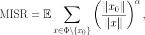
That said, there is a quantity that is very useful when it has a finite mean: the interference-to-(average)-signal ratio ISR, defined as

$\displaystyle {\rm ISR}=\frac{\sum_{x\in\Phi\setminus\{x_0\}} h_x \|x\|^{-\alpha}}{\|x_0\|^{-\alpha}},$

where x₀ is the desired transmitter and the other points of Φ are interferers. The h_x are the fading random variables (assumed to have mean 1), only present in the numerator (interference), since the signal power here is averaged over the fading.
Taking the expectation of the ISR eliminates the fading, and we arrive at the mean ISR

$\displaystyle {\rm MISR}=\mathbb{E} \sum_{x\in\Phi\setminus\{x_0\}}\left(\frac{\|x_0\|}{\|x\|}\right)^{\alpha},$

which only depends on the network geometry. It follows that the SIR distribution is

$\displaystyle \mathbb{P}({\rm SIR}<\theta)=\mathbb{P}(h<\theta\, {\rm ISR})=\mathbb{E} F_h(\theta\,{\rm ISR}),$

where h is a generic fading random variable. If h is exponential (Rayleigh fading) and the MISR is finite,

$\displaystyle F_h(x)\sim x\qquad\Longrightarrow\qquad \mathbb{P}({\rm SIR}<\theta)\sim \theta\,{\rm MISR}.$

Hence for small θ, the outage probability is proportional to θ with proportionality factor MISR. This simple fact becomes powerful in conjunction with the observation that in cellular networks, the SIR distributions (in dB) are essentially just shifted versions of the basic SIR distribution of the PPP (and of each other).

Figure 1: Examples for SIR distributions in cellular networks that are essentially shifted versions of each other.

In Fig. 1, the blue curve is the standard SIR ccdf of the Poisson cellular network, the red one is that of the triangular lattice, which has the same shape but shifted by about 3 dB, with very little dependence on the path loss exponent. The other two curves may be obtained using base station silencing and cooperation, for instance. Since the shift is almost constant, it can be determined by calculating the ratios of the MISRs of the different deployments or schemes. The asymptotic gain relative to the standard Poisson network (as θ→0) is

$\displaystyle G_0=\frac{\rm MISR_{PPP}}{{\rm MISR}},\quad \text{where }\; {\rm MISR_{PPP}}=\frac{2}{\alpha-2},\quad \alpha>2,$

The MISR in this expression is the MISR for an alternative deployment or architecture. The MISR for the PPP is not hard to calculate. Extrapolating to the entire distribution by applying the gain everywhere, we have

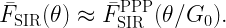
$\displaystyle \bar F_{\rm SIR}(\theta) \approx \bar F_{\rm SIR}^{\rm PPP}(\theta/G_0).$

This approach of shifting a baseline SIR distribution was proposed here and here. It is surprisingly accurate (as long as the diversity order of the transmission scheme is unchanged), and it can be extended to other types of fading. Details can be found here.

Hence there are good reasons to focus on the reversed SIR, i.e., the ISR.

Stogblog by M. Haenggi

Signal-to-interference, reversed

Leave a Reply Cancel reply

Share this:

Like this:

Related

Leave a Reply Cancel reply