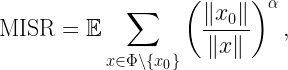
In performance analyses of wireless networks, we frequently encounter expectations of the form

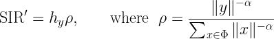
called average (ergodic) spectral efficiency (SE) or mean normalized rate or similar, in units of nats/s/Hz. For networks models with uncertainty, its evaluation requires the use stochastic geometry. Sometimes the metric is also normalized per area and called area spectral efficiency. The SIR is expressed in the form
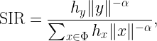
with Φ being the point process of interferers.
There are several underlying assumption made when claiming that (*) is a relevant metric:
- It is assumed that codewords are long enough and arranged in a way (interspersed in time, frequency, or across antennas) such that fading is effectively averaged out. This is reasonable for several current networks.
- It is assumed that desired signal and interference amplitudes are Gaussian. This is sensible since if a decoder is intended for Gaussian interference, then the SE is as if the interference amplitude were indeed Gaussian, regardless of its actual distribution.
- Most importantly and questionably, taking the expectation over all fading random variables hx implies that the receiver has knowledge of all of them. Gifting the receiver with all the information of the channels from all interferers is unrealistic and thus, not surprisingly, leads to (*) being a loose upper bound on what is actually achievable.
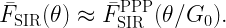
So what is a more realistic and accurate approach? It turns out that if the fading in the interferers’ channels is ignored, i.e., by considering
we can obtain a tight lower bound on the SE instead of a loose upper bound. A second key advantage is that this formulation permits a separation of temporal and spatial scales, in the sense of the meta distribution. We can write
is a purely geometric quantity that is fixed over time and cleanly separated from the time-varying fading term hy. Averaging locally (over the fading), the SE follows as

which is a function of (conditioned on) the point process. For instance, with Rayleigh fading,
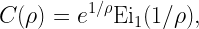
where Ei1 is an exponential integral. The next step is to find the distribution of ρ to calculate the spatial distribution of the SE – which would not be possible from (*) since it is an “overall average” that lumps all randomness together. In the case of Poisson cellular networks with nearest-base station association and path loss exponent 2/δ, a good approximation is
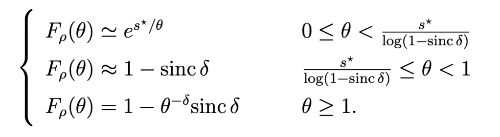
Here s* is given by
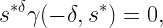
and γ is the lower incomplete gamma function. This approach lends itself to extensions to MIMO. It turns out that the resulting distribution of the SE is approximately lognormal, as illustrated in Fig. 1.

For SISO and δ=1/2 (a path loss exponent of 4), this (approximative) analysis shows that the SE achieved in 99% of the network is 0.22 bits/s/Hz, while a (tedious) simulation gives 0.24 bits/s/Hz. Generally, for small ξ, 1/ln(1/ξ) is achieved by a fraction 1-ξ of the network. As expected from the discussion above, this is a good lower bound.
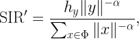
In contrast, using the SIR distribution directly (and disregarding the separation of temporal and spatial scales), from

we would obtain an SE of only log2(1.01)=0.014 bits/s/Hz for 99% “coverage”, which is off by a factor of 16! So it is important that coverage be gleaned from the ergodic SE rather than a quantity subject to the small-scale variations of fading. See also this post.
The take-aways for the ergodic spectral efficiency are:
- Avoid mixing time and spatial scales by expecting first over the fading and separately over the point process; this way, the spatial distribution of the SE can be obtained, instead of merely its average.
- Avoid gifting the receiver with information it cannot possibly have; this way, tight lower bounds can be obtained instead of loose upper bounds.
The details can be found here.