Intuition may tell us that increasing the randomness in the system (e.g., by increasing the variance of some random variables relative to their mean) will decrease the correlation between some random quantities of interest. A prominent example is the interference or SIR in a wireless network measured at two locations or in two time slots.

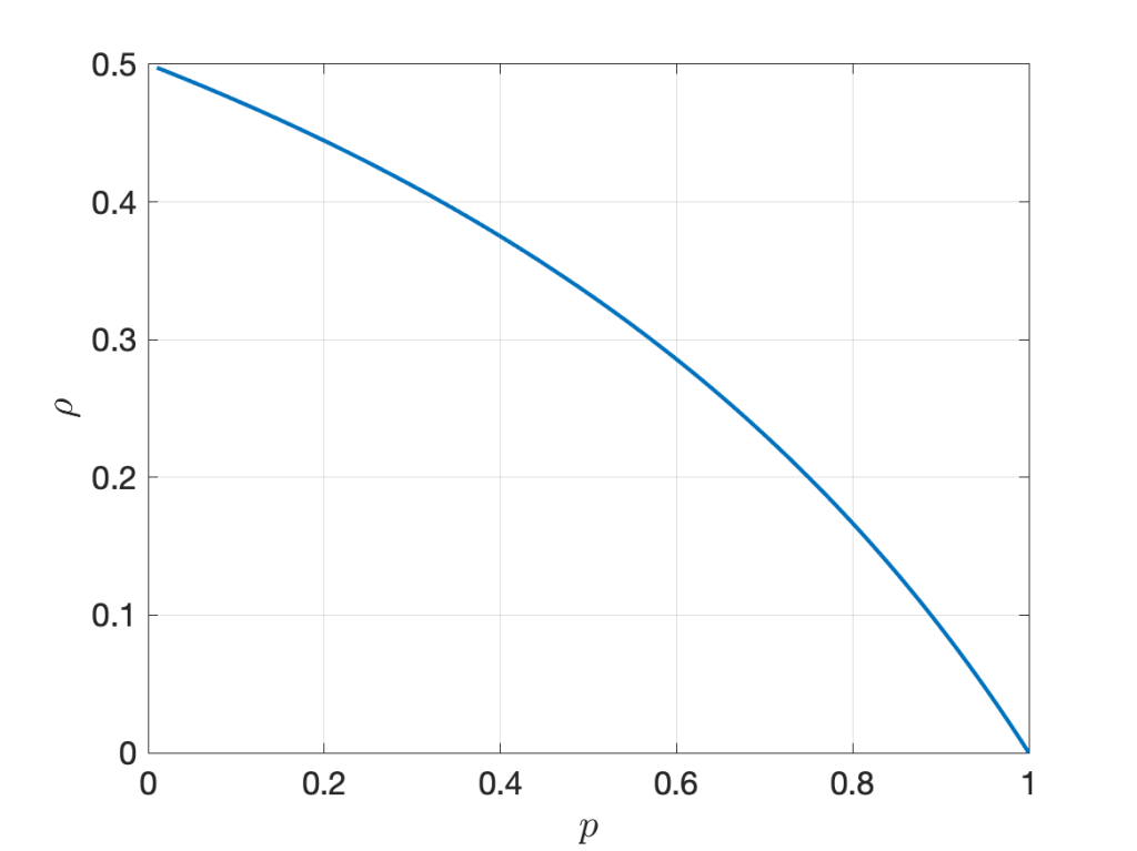
Let us consider a simple example to explore whether this intuition is correct. We consider the two random variables XY₁ and XY₂, where Y₁ and Y₂ are iid exponential with mean 1 and X is Bernoulli with mean p, independent of the Y_k. In this case, Pearson’s correlation coefficient is

It is illustrated in Figure 1 below. The randomness in X, measured by the ratio of variance to mean, is 1-p . However, increasing the randomness monotonically increases the correlation. As p approaches 0, the correlation tends to its maximum of 1/2.

Next, let Y₁ and Y₂ be independent and Bernoulli with mean p and X gamma distributed with parameters m and 1/m, such that the mean of X is 1 and the variance 1/m. Again we focus on the correlation of the two products XY₁ and XY₂. In this case, the correlation coefficient is

shown in Figure 2 below for different values of m. Again, we observe that increasing the randomness in X (decreasing m) increases the correlation for all p <1. For p =1, the correlation is 1 since both random variables equal X.

So is the relationship between randomness and correlation completely counter-intuitive? Not quite, but our intuition is probably skewed towards the case of independent randomness, as opposed to common randomness. In the second example, the randomness in Y₁ and Y₂ decreases with p, and the correlation coefficient increases with p, as expected. Here Y₁ and Y₂ are independent. In contrast, X is the common randomness. If its variance increases, the opposite happens – the randomness decreases.

In the wireless setting, the common randomness is often the point process of transceiver locations, while the independent randomness usually comprises the fading coefficients and the channel access indicators. One of the earliest results on correlations in wireless networks is the following: For transmitters forming a PPP, with each one being active independently with probability p in each time slot (slotted ALOHA) and independent Nakagami-m fading, the correlation coefficient of the interference measured at the same location in two different time slots is (see Cor. 2 in this paper)

Here the fading coefficients have the same gamma distribution as in the second example above. As expected, increasing the randomness in the channel access (decreasing p) and in the fading (decreasing m) both reduce the correlation. Conversely, setting p =1 and letting m → ∞, the correlation coefficient is 1. However, the correlation is induced by the PPP as the common randomness – if the node placement was deterministic, the correlation would be 0. In other words, the interference in different times slots is conditionally independent given the PPP. This conditional independence is exploited in the analysis of important metrics such as the local delay and the SIR meta distribution.

One last remark. The expression (*) shows that the correlation coefficient is simply the product of the transmit probability p and the Nakagami fading parameter m mapped to the (0,1) interval using the Möbius homeomorphic transform described here, which is m /(m+1). This shows a nice symmetry in the impact of channel access and fading.

• Misconceptions
• Other points