In this post I would like to show how meta distributions naturally emerge as an important extension of the concepts of averages and distributions. For a random variable Z, we call 𝔼(Z) its average (or mean). If we add a parameter z to compare Z against and form the family of random variables 1(Z>z), we call their mean the distribution of Z (to be precise, the complementary cumulative distribution function, ccdf for short).
Now, if Z does not depend on any other randomness, then 𝔼1(Z>z) gives the complete information about all statistics of Z, i.e., the probability of any event can be expressed by adding or subtracting these elementary probabilities.
However, if Z is a function of other sources of randomness, then 𝔼1(Z>z) does not reveal how the statistics of Z depend on those of the individual random elements. In general Z may depend on many, possibly infinitely many, random variables and random elements (e.g., point processes), such as the SIR in a wireless network. Let us focus on the case Z=f(X,Y), where X and Y are independent random variables. Then, to discern how X and Y individually affect Z, we need to add a second parameter, say x, to extend the distribution to the meta distribution:
![\displaystyle \bar F_{[\![Z\mid Y]\!]}(z,x)=\mathbb{E}\mathbf{1}(\mathbb{E}[\mathbf{1}(Z>z) \mid Y]>x).](https://s0.wp.com/latex.php?latex=%5Cdisplaystyle+%5Cbar+F_%7B%5B%5C%21%5BZ%5Cmid+Y%5D%5C%21%5D%7D%28z%2Cx%29%3D%5Cmathbb%7BE%7D%5Cmathbf%7B1%7D%28%5Cmathbb%7BE%7D%5B%5Cmathbf%7B1%7D%28Z%3Ez%29+%5Cmid+Y%5D%3Ex%29.&bg=ffffff&fg=000000&s=2&c=20201002)
Alternatively,
![\displaystyle \bar F_{[\![Z\mid Y]\!]}(z,x)=\mathbb{E}\mathbf{1}(\mathbb{E}_X\mathbf{1}(Z>z)>x).](https://s0.wp.com/latex.php?latex=%5Cdisplaystyle+%5Cbar+F_%7B%5B%5C%21%5BZ%5Cmid+Y%5D%5C%21%5D%7D%28z%2Cx%29%3D%5Cmathbb%7BE%7D%5Cmathbf%7B1%7D%28%5Cmathbb%7BE%7D_X%5Cmathbf%7B1%7D%28Z%3Ez%29%3Ex%29.&bg=ffffff&fg=000000&s=2&c=20201002)
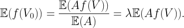
Hence the meta distribution (MD) is defined by first conditioning on part of the randomness. It has two parameters, the distribution has one parameter, and the average has zero parameters. There is a natural progression from averages to distributions to meta distributions (and back), as illustrated in this figure:

From the top going down, we obtain more information about Z by adding indicators and parameters. Conversely, we can eliminate parameters by integration (taking averages). Letting U be the conditional ccdf given Y, i.e., U=𝔼X1(Z>z)=𝔼[1(Z>z) | Y], it is apparent that the distribution of Z is the average of U, while the MD is the distribution of U.
Let us consider the example Z=X/Y , where X is exponential with mean 1 and Y is exponential with mean 1/μ, independent of X. The ccdf of Z is

In this case, the mean 𝔼(Z) does not exist. The conditional ccdf given Y is the random variable

and its distribution is the meta distribution
![\displaystyle \bar F_{[\![Z\mid Y]\!]}(z,x)\!=\!\mathbb{P}(U\!>\!x)\!=\!\mathbb{P}(Y\!\leq\!-\log(x)/z)\!=\!1\!-\!x^{\mu/z}.](https://s0.wp.com/latex.php?latex=%5Cdisplaystyle+%5Cbar+F_%7B%5B%5C%21%5BZ%5Cmid+Y%5D%5C%21%5D%7D%28z%2Cx%29%5C%21%3D%5C%21%5Cmathbb%7BP%7D%28U%5C%21%3E%5C%21x%29%5C%21%3D%5C%21%5Cmathbb%7BP%7D%28Y%5C%21%5Cleq%5C%21-%5Clog%28x%29%2Fz%29%5C%21%3D%5C%211%5C%21-%5C%21x%5E%7B%5Cmu%2Fz%7D.&bg=ffffff&fg=000000&s=2&c=20201002)
As expected, the ccdf of Z is retrieved by integration over x∈[0,1]. This MD has relevance in Poisson uplink cellular networks, where base stations (BSs) form a PPP Φ of intensity λ and the users are connected to the nearest BS. If the fading is Rayleigh fading and the path loss exponent is 2, the received power from a user at an arbitrary location is S=X/Y, where X is exponential with mean 1 and Y is exponential with mean 1/(λπ), exactly as in the example above. Hence the MD of the signal power S is
![\displaystyle \qquad\qquad\qquad\bar F_{[\![S\mid \Phi]\!]}(z,x)=1-x^{\lambda\pi/z}.\qquad\qquad\qquad (1)](https://s0.wp.com/latex.php?latex=%5Cdisplaystyle+%5Cqquad%5Cqquad%5Cqquad%5Cbar+F_%7B%5B%5C%21%5BS%5Cmid+%5CPhi%5D%5C%21%5D%7D%28z%2Cx%29%3D1-x%5E%7B%5Clambda%5Cpi%2Fz%7D.%5Cqquad%5Cqquad%5Cqquad+%281%29&bg=ffffff&fg=000000&s=2&c=20201002)
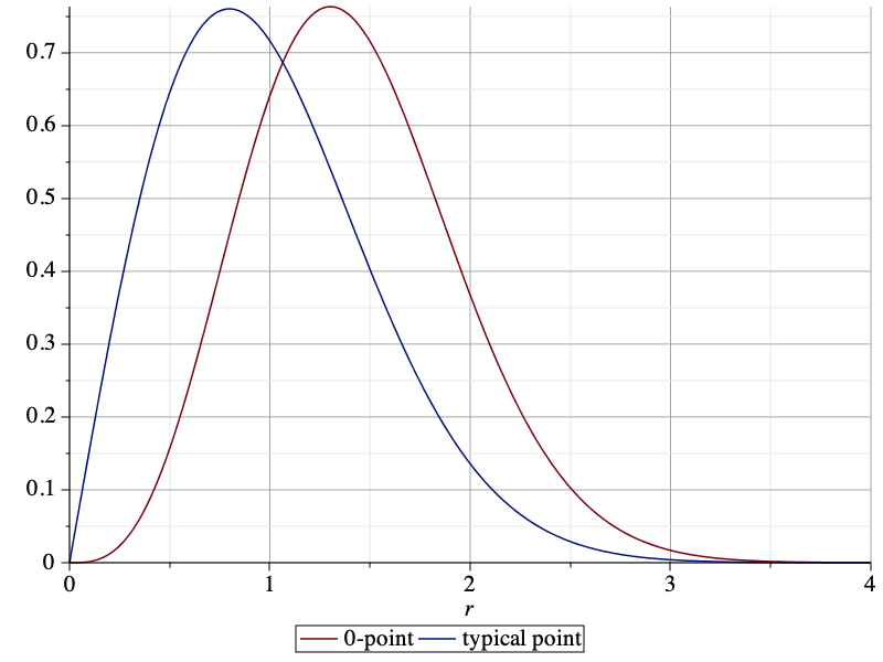
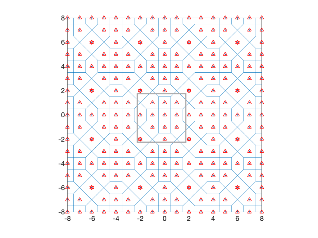
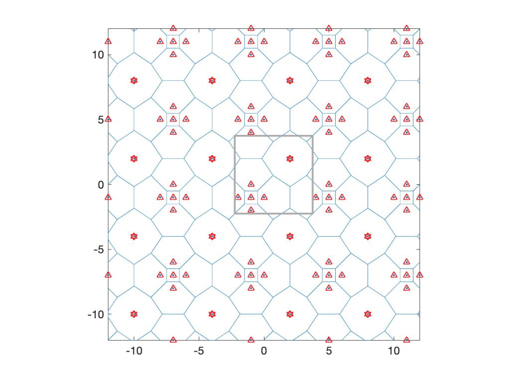
So what additional information do we get from the MD, compared to just the ccdf of S? Let us consider a realization of Φ and a set of users forming a lattice (any stationary point process of users would work) and determine each user’s individual probability that its received power exceeds 1:

If we draw a histogram of all the user’s probabilities (the numbers in the figure), how does it look? This cannot be answered by merely looking at the ccdf of S. In fact ℙ(S>1)=π/(π+1)≈0.76 is merely the average of all the numbers. To know their distribution, we need to consult the MD. From (1) the MD (for λ=1 and z=1) is 1-xπ. Hence the histogram of the numbers has the form of the probability density function πxπ-1. In contrast, without the MD, we have no information about the disparity between the users. Their personal probabilities could all be well concentrated around 0.76, or some could have probabilities near 0 and others near 1. Put differently, only the MD can reveal the performance of user percentiles, such as the “5% user” performance, which is the performance that 95% of the users achieve but 5% do not.
This interpretation of the MD as a distribution over space for a fixed realization of the point process is valid whenever the point process is ergodic.
Another application of the MD is discussed in an earlier post on the fraction of reliable links in a network.