When applying simalysis as illustrated in the previous post, the question arises where to put the boundary between the part of the point process that is simulated and the part that is analyzed. Specifically, we may wonder whether we can reduce the simulated part to only a single point (on average), i.e., to choose the number of simulated points to be Poisson with mean 1 in each realization.
Let’s find out, using the same Poisson bipolar model as in the previous post (Rayleigh fading, transmitter density 1, link distance 1/4).

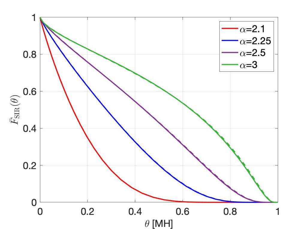
Fig. 1 shows the simulated (or, more precisely, simalyzed) result where the 500 realizations only contain one single point on average. This means that about 500/e ≈ 184 realizations have no point at all. We observe good accuracy, especially at small path loss exponents α. Also, the simulated curves are lower bounds to the exact ones. This is due to Jensen’s inequality:

The term on the left side is the exact factor in the SIR ccdf due to the interference I_c from points outside distance c. It is larger than the right side, which is the factor used in the simalysis (see the Matlab code). This property holds for all stationary point processes.

But why stop there? One would think that using, say, only 1/4 point on average would be (essentially) pointless. But let’s try, just to be sure.

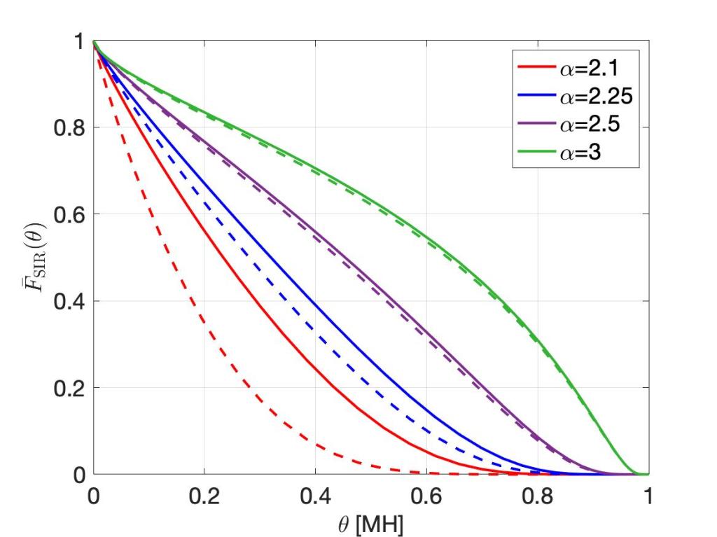
Remarkably, even with only 1/4 point per realization on average, the curves for α<2.5 are quite accurate, and the one for α=2.1 is an excellent lower bound! It is certainly much more accurate than a classical simulation with 500,000 points per realization (see the previous post). Such a good match is quite surprising, especially considering that 1/4 point on average means that about 78% of the realizations have 0 points, which means that in about 390 out of the 500 realizations, the simulated factor in the SIR ccdf simply yields 1. Also, in the entire simalysis, only about 125 points are ever produced. It takes no more than about 1/2 s on a standard computer.
We conclude that accurate simulation (simalysis, actually) can be almost point-less.

Simulations can be quite time-consuming. Are there any techniques that can help make them more efficient and/or accurate? Let us focus on a concrete problem. Say we would like to plot the SIR distribution in a Poisson bipolar network for different path loss exponents α, including some values close to 2. Since we would like to compare the result with the exact one, we focus on the Rayleigh fading case where the analytical expression is known and simple. The goal is to get accurate curves for α=3, 2.5, 2.25, and 2.1, and we would like to wait no longer than 1 s for the results on a standard desktop or laptop computer.
Let us first discuss why this is a non-trivial problem. It involves averaging w.r.t. the fading and the point process, and we need to make sure that the number of interferers is large enough for good accuracy. But what is “large enough”? A quick calculation using Campbell’s theorem (for sums) reveals that if we want to capture 99% of the mean interference power (outside radius 1 to avoid complications due to a potential singularity in the path loss law), we find that for α=3, the simulation region needs to be 100 times larger than for α=4. This seems manageable, but for α=2.5, 2.25, 2.1, it is 10⁶, 10¹⁴, 10³⁸ times larger, respectively!
Clearly the straightforward approach of producing many realizations of the PPP in a large region does not work in the regime of small α. So how can we achieve our goal above – high accuracy and high efficiency?

The solution is to use an analysis-enhanced simulation technique, which I call simalysis. While we often tend to think as analysis vs. simulation as a dichotomy, in this approach they are used symbiotically. The idea is to exploit analytical results whenever possible to make simulations faster and more accurate. Let me illustrate how simalysis works when applied to the problem above.

For small α, it is impossible to “capture” most of the interference solely by simulation. In fact, most of it stems from the infinitely many distance nodes, each one contributing little, with independent fading. We can thus assume that the variance of the interference of the nodes further than a certain distance (relatively large compared with the mean nearest-neighbor distance) is relatively small. Accordingly, replacing it by its mean is a sensible simplification. Here is where the analysis comes in. For any stationary point process of density λ, the mean interference from the nodes outside distance c is

This interference term can then be added to the simulated interference, which stems from points within distance c. Simulating as few as 50 points is enough for very high accuracy. The result is shown in the figure below, using the MH scale so that the entire distribution is revealed (see this post for details on the MH scale). For α near 2, the curves are indistinguishable!

This simulation averages over 500 realizations of the PPP and runs in less than 1 s on a laptop. The Matlab code is available here. It uses a second simalytic technique, namely the analytical averaging over the fading. Irrespective of the type of point process we want to simulate, as long as the fading is Rayleigh, we can perform the averaging over the fading analytically.

For comparison, the figure below shows the simulation results if 500,000 points (interferers) are simulated, without adding the analytical mean interference term, i.e., using classical simulation. Despite taking 600 times longer, the distributions for α<2.5 are not acceptable.