Papers on wireless networks frequently present analytical approximations of distributions. The reference (exact) distributions are obtained either by simulation or by the numerical evaluation of a much more complicated analytical expression. The approximation and the reference distributions are then plotted, and a “highly accurate” or “extremely precise” match is usually declared. There are several issues with this approach.
First, people disagree on what “highly accurate” means. If there is a yawning gap between the distributions, can (should) the match be declared “very precise”? Without any quantification of what “accurate” or “precise” means, it is hard to argue one way or another.
Second, the visual impression can be distorted due to the use of a logarithmic (dB) scale and since, if the distribution has infinite support, only part of it can ever be plotted.
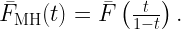
In this post I suggest an approach that addresses both these issues, assuming that at least one of the distributions in question is only available in numerical form (discrete data points). For the second one, we use the Möbius homeomorphic transform to map the infinite support to the [0,1] unit interval. Focusing on complementary cumulative distributions (ccdfs) and assuming the original distribution is supported on the positive real line, the mapped ccdf is obtained by
The MH transform and its advantages are discussed in this blog. For instance, it is very useful when applied to SIR distributions. In this case, the mapped ccdf is that of the signal fraction (ratio of desired signal power to total received power). For our purposes here, the [0,1] support is key as it allows not only a complete visualization but also lends itself as a natural distance metric that is itself normalized to [0,1]. Here is the definition of the MH distance:

Trivially it is bounded by 1, so the distance value directly and unambiguously measures the match between the ccdfs. Accordingly, we can use terms such as “mediocre match” or “good match” depending on this distance. The terminology should be consistent with the visual impression. For instance, if the MH ccdfs are indistinguishable, the match should be called “perfect”. Therefore, to address the first issue raised above, I propose the following intervals and terms.
| term for match | range |
| bad | 0.05 – 1 |
| mediocre | 0.02 – 0.05 |
| acceptable | 0.01 – 0.02 |
| good | 0.005 – 0.01 |
| excellent | 0.002 – 0.005 |
| perfect | 0 – 0.002 |
Another advantage of the MH distance is that it emphasizes the high-value regime (the ccdf near 0) over the low-value regime since it maps values near 0 without distortion while it compresses high values. In the case of SIR ccdfs whose value indicate reliabilities, high values mean high reliabilities, which is the relevant regime in practice.
A simple Matlab implementation of the MH distance is available here. It accepts arbitrary values of the ccdf’s arguments and uses interpolation to achieve uniform sampling of the [0,1] interval.
As an example, here is an animation showing a standard exponential ccdf (MH mapped of course) in blue and another exponential ccdf with a parameter varying from 1.5 to 0.64. It is apparent that the terminology corresponds to the visual appraisal of the gap between the two ccdfs.


@Prof. Haenggi: Given that there are well-established metrics (Kolmogorov distance or more importantly Wasserstein distance comes to mind) to measure the “distance” between distributions, is there any additional benefit that the MH distance brings? More precisely, why transform first before measuring the distances? Maybe so as to harmonize all metrics/parameters?
One interesting question might be whether the MH distance is bounded below/above etc as compared to K-distance or W-distance.
LikeLike
The Wasserstein-1 distance of the MH mapped distributions corresponds to the MH distance (both are defined as L1 norms). Similar to the general Wasserstein distance, the MH distance could be extended to different norms.
Secondly, if you don’t transform first you need to integrate (or sum) over an infinite range plus you get a result that is not bounded. Say the distance is 230. There is no way to tell. With the MH distance you immediately know from the value whether it is an accurate match or not. Lastly, it is satisfactory if the terminology agrees with the visual impression. Since the ccdf with infinite support cannot be plotted entirely, there could be perfect agreement in the range shown but a significant gap in the part that is not shown.
LikeLike